
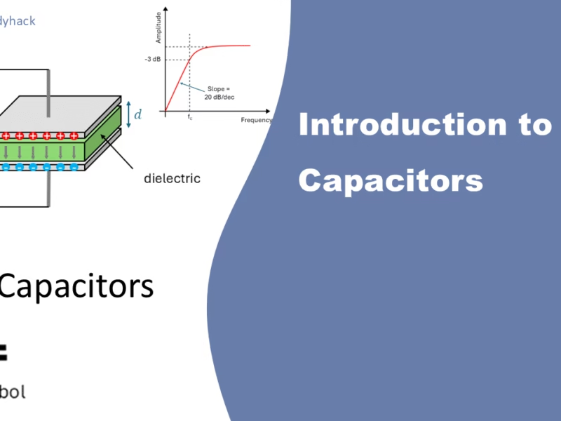
1. Introduction to capacitors
In this tutorial on capacitors, we will explore the fundamentals of these essential passive electronic components. Capacitors are composed of two or more conductive materials separated by an insulating dielectric. They have the unique ability, or “capacity,” to store energy in the form of electrical charge, which creates a potential difference (or static voltage) across their plates.
We will begin by discussing the construction and operation of capacitors, providing insight into how they function. Next, we will examine the process of applying DC voltage to charge and discharge a capacitor. Finally, we will explore the application of AC voltages, particularly in the context of high-frequency signals within low- and high-pass filter systems.
2. Capacitor
A capacitor consists of two conductive plates separated by a dielectric, which is an insulating material. The dielectric can be air, ceramic, plastic, paper, or other materials that prevent direct current (DC) from flowing through the capacitor. This layer is essential, as it allows a voltage to develop across the plates by holding an electric charge rather than letting current flow between them.
When a capacitor is placed in a DC circuit, it charges up to match the supply voltage, and once charged, it effectively blocks the flow of current. In an alternating current (AC) circuit, however, the capacitor behaves differently. Since AC constantly changes direction, the capacitor repeatedly charges and discharges, creating an effect that lets AC current “pass through” the capacitor. This makes capacitors useful in various applications like filtering, signal coupling, and energy storage. The exact effect of an AC signal on the capacitor, I discuss in the chapter on filters.
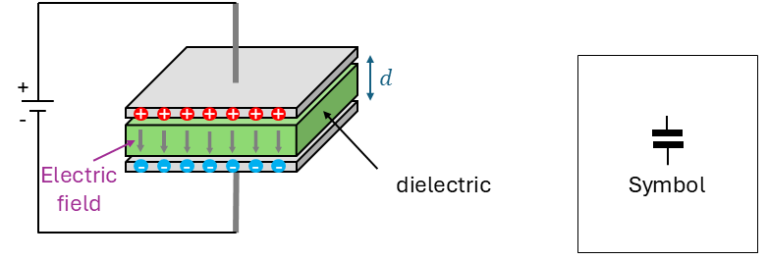
The capacitance of a capacitor, measured in Farads (F), depends on several factors: the area of the conductive plates, the thickness and type of dielectric material, and the separation distance between the plates. A larger plate area or a smaller gap between the plates increases capacitance, allowing the capacitor to store more charge at a given voltage.
This stored charge generates an electrostatic field in the dielectric, effectively storing energy that can later be released. The ratio of stored charge Q to the applied voltage V gives the capacitance C, expressed by C=Q/V. This property of capacitance allows the capacitor to resist sudden changes in voltage across it, making it valuable in circuits for smoothing voltage or providing bursts of power when needed.
While we often describe the charge as being held on the plates, the energy is more accurately stored in the electric field between them. As current flows into the capacitor, the field strengthens, and as it discharges, the field weakens, releasing stored energy back into the circuit. Capacitors thus play a crucial role in both storing and regulating electrical energy, essential in electronics and power systems.
2.1 Dielectric
The dimension and material of the capacitor also play a crucial role in the capacitance of the capacitor. The capacitance is directly proportional to the area of the conductive plate, and inversely proportional to the distance between the plates. The capacitance formula for such a capacitor is give by
\[C=\varepsilon\frac{A}{d}\]
where ε represents the absolute permittivity of the dielectric material, A is the area of the conductive plate, and d is the distance between them. The permittivity of the dielectric material, includes the permittivity of free space, ε0 and the relative permittivity εr (also known as dielectric constant), which measures how much the dielectric increases capacitance compared to vacuum (εr for air = 1). The capacitors effective permittivity is calculcated by ε = ε0/εr.
For two plates of 2cm by 10cm, separated by air with a distance of 1mm, we can calculate the capacitance as follows:
\[C=\varepsilon_0\varepsilon_r\frac{A}{d} = 8.854\times 10^{-12}\times 1\frac{0.02\times 0.1}{0.001} = 1.77\times 10^{-11} F = 17.7 pF\]
2.1.1 Capacitance in Farad
The capacitance is the measure of a capacitor’s ability to store electrical charge onto its plates. The unit of capacitance is Farad (abbreviated to F), named after the physicist M. Faraday. 1 Farad means it can store 1 Coulomb of charge across a potential difference of 1 Volt.
Normally, this is such a large unit that you will typically see units in the range of pico-farads (pF), nano-farads (nF) or micro-farads (μF).
2.1.2 Energy in a capacitor
When a capacitor is fully charged by a power supply, it creates an electric field that stores energy. The amount of energy stored in joules (J) is equal to the work done by the voltage supply to maintain the charge on the capacitor’s plates, and is given by the equation:
\[W = \frac{1}{2}CV^2 \text{(J)}\]
In this sense, a capacitor resembles a battery. While a battery stores energy through electrochemical reactions, a capacitor stores its energy as electrostatic energy in an electric field. One significant difference between the two is the rate at which they discharge energy: a capacitor can charge and discharge much faster than a battery, but it cannot maintain a constant voltage over an extended period.
3. Charging/discharging a capacitor
The Figure below illustrates an RC circuit, where a capacitor (C) is in series with a resistor (R) and connected to a battery power supply (Vs) through a mechanical switch. At the instant the switch is closed, the capacitor starts charging through the resistor. This charging process continues until the capacitor’s voltage equals the battery’s supply voltage.

Let us assume initially that the capacitor C is fully discharged and the switch is open. These are the initial conditions for the circuit, where t=0, i=0, q=0. When the switch is closed, time starts at t=0, and current begins flowing into the capacitor through the resistor.
Since the initial voltage across the capacitor is zero (Vc=0 at t=0), the capacitor initially behaves like a short circuit relative to the external circuit. This allows the maximum current to flow, limited only by the resistor R, with i=Vs/R.
As the capacitor starts charging, charge builds up on its plates, creating an increasing voltage Vc that opposes the battery voltage Vs. This opposition reduces the current gradually as the capacitor voltage Vc approaches Vs, resulting in an exponential decrease in current over time.
This charging behavior follows a time constant, represented by:
\[\tau = RC\]
where R is in Ohms and C in Farads. The time constant τ represents the time required for the capacitor to reach approximately 63% of its final charge, or equivalently for the current to fall to about 37% of its initial value. The value of τ depends on the resistance R and capacitance C: a larger R slows the charging rate, while a larger C allows the capacitor to hold more charge, also requiring more time to reach full charge.

As charging progresses, the voltage across the capacitor follows an RC charging curve, rising sharply at first and then leveling off as it approaches Vs. At one time constant, 1τ, the capacitor reaches 63% of Vs. Over approximately five time constants, or 5τ, the capacitor is essentially fully charged, with the current approaching zero and the voltage across the capacitor equaling Vs.
At this final stage (theoretically at t=∞), the capacitor behaves like an open circuit, holding the full supply voltage across it, while current i falls to zero, and the total charge reaches Q=CV.
3.1 RC Time constant
The voltage across the capacitor Vc at time t, while it is charging, can be calculated by the formula:
\[Vc = Vs\left(1-e^{-\frac{t}{RC}}\right)\]
where Vs is the supply voltage, e ≈ 2.718 is Euler’s number, t is the time elapsed since the switch was closed, and RC is the time constant τ of the RC circuit.
As time progresses, the voltage across the capacitor follows an exponential curve, increasing quickly at first and slowing as it approaches Vs. At around 5 time constants (5τ), the capacitor voltage has essentially reached Vs, and we consider it fully charged. At this point, known as the Steady State Period, the charging current i becomes zero, and no further current flows in the circuit, as Vc ≈ Vs.
Note that theoretically, the capacitor never reaches 100% fully charged. Even after 5τ, it only reaches 99.3%, as shown in the table below. For all practical purposes, we can consider this point to be fully charged, as there will be hardly any change after this.
| Time constant | Voltage |
| 0.5 τ | 39.3% |
| 0.7 τ | 50.3% |
| 1 τ | 63.2% |
| 2 τ | 86.5% |
| 3 τ | 95.0% |
| 4 τ | 98.2% |
| 5 τ | 99.3% |
4. Filter Circuits
The statement that capacitors passes AC and blocks DC is not so simplistic. In the previous sections we mentioned that capacitors have a time constant and if you change the capacitance, you change the time constant. Now, there is a relation between time and (angular) frequency, which is that frequency is the reciprocal of time (ω = 1/RC). So if you change the value of a capacitor, you also change the frequency of the circuit the capacitor is in. A given capacitor will pass all frequencies above a certain frequency and block all signals below that frequency.
As an example, an RC circuit with a 100-ohm resistor and a 33-picofarad capacitor, the cutoff frequency (fc) is approximately:
\[f_c = \frac{\omega}{2\pi}=\frac{1}{2\pi RC} = \frac{1}{2\pi\times 100\times 33\times 10^{-12}} \approx 48.2 MHz\]
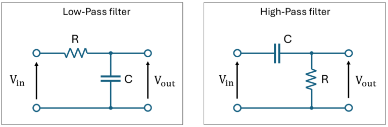
The question now is, where does it passes the signals to? This depends entirely on the placement of the capacitor in the RC circuit.
- Low-pass filter: If the capacitor is placed parallel to the signal flow, with its lead to the ground, it will pass the 48.2 MHz signal to ground, effectively blocking the signal (and all higher frequencies) from the going to the next stage.
- High-pass filter: If the capacitor is placed in series with the signal flow, it will allow the 48.2 MHz (and higher frequencies) signal to pass to the next stage, and blocking all signals below that frequency.
4.1 Transfer function
The explanation above provides a more intuitive, “hand-waving” approach to understanding low-pass and high-pass filters. However, to analyze these filters rigorously, we use transfer functions and apply Laplace transformations.
For example the high-pass filter, we can write the input-output (vi /vo) equations as follows:
\[v_i(t) = v_C(t)+v_R(t)\]
\[v_o(t) = v_R(t)\]
considering that i(t) is the current through the circuit (no load) and vC(t) is the voltage across C:
\[v_i(t)=\frac{1}{C}\int i(t)dt + Ri(t)\]
\[v_o(t)=Ri(t)\]
applying the Laplace transformation on the input voltage, where I(s) is the Laplacian of i(t):
\[V_i(s) = \frac{1}{sC}I(s)+RI(s) = I(s)\left(R+\frac{1}{sC}\right) \]
therefore
\[I(s)=\frac{V_i(s)}{R+\frac{1}{sC}}\]
The Laplace transformation for the output yields:
\[V_o(s) =RI(s)=\frac{V_i(s)R}{R+\frac{1}{sC}}\]
Therefore, the transfer function H is:
\[H(s) = \frac{V_o(s)}{V_i(s)}=\frac{R}{R+\frac{1}{sC}}=\frac{R}{\frac{sRC+1}{sC}}=\frac{sRC}{sRC+1}=\frac{s}{s+\frac{1}{RC}}\]
4.2 Frequency response analysis
To look at the filter in the frequency domain, we substitute s= jω, where ω=2πf.
\[H(j\omega )=\frac{j\omega}{j\omega+\omega_c}\]
where ωc = 1/RC.
To further analyze how this filter responds to different input frequencies, we can use a Bode plot as a graphical tool. A Bode plot consists of two parts: a magnitude plot, which displays the gain (or amplitude) of the output as a function of frequency, and a phase plot, which shows how much the output signal lags or leads the input signal at each frequency. Together, these plots provide insight into the filter’s behavior across frequencies, revealing its characteristics, stability, and any resonant frequencies.
4.2.1 Magnitude plot
The magnitude of H(jω) is:
\[|H(j\omega)|=\left|\frac{j\omega}{j\omega+\frac{1}{RC}}\right|=\frac{\omega}{\sqrt{\omega^2+\left(\frac{1}{RC}\right)^2}}\]
Convert this to decibels (dB) for the Bode magnitude plot:
\[20\text{log}_{10}(|H(j\omega)|)=20\text{log}_{10}\left(\frac{\omega}{\sqrt{\omega^2+\left(\frac{1}{RC}\right)^2}}\right)\]
at lower frequencies (ω << ωc), the gain decreases at a rate of -20 dB/decade below the cutoff frequency fc, attenuating lower frequencies significantly. At higher frequencies (ω >> ωc), the magnitude asymptotically approaches 0 dB, meaning the high-pass filter passes these frequencies with little or no attenuation.

4.2.2 Phase plot
The phase of H(jω) is:
\[\phi(\omega) = 90^o-\text{tan}^{-1}\left(\frac{\omega}{\omega_c}\right)\]
at lower frequency (ω << ωc), the phase is 90°; when ω = ωc the phase is 45°; and at higher frequency (ω >> ωc), the phase reaches 0°.

5. References
- The Arts of Electronics – P. Horowitz & W. Hill, third edition (2015).
- Introduction to charging an RC circuit
- A very basic introduction to Capacitors
- Fundamentals of RC filters
- Poles and zeros for Laplace transformation of a low-pass filter.
Florius
Hi, welcome to my website. I am writing about my previous studies, work & research related topics and other interests. I hope you enjoy reading it and that you learned something new.
More Posts