

1. Ferromagnetic Resonance (FMR): Theoretical framework
In the previous posts on the LLG equation and Spin-torque transfer, I discussed how the precession of the magnetization is governed by the Larmor precession and the Gilbert relaxation damping. In order to experimentally measure this relaxation, an oscillating magnetic field (hrf) is applied to the sample with a certain frequency (ω=2πf), perpendicular to the external magnetic DC field (H0). the small oscillating magnetic field causes the magnetization to get out of its equilibrium position, and making it rotate around the effective field (Heff). Figure 1 illustrates how the magnetization of the sample is processing under these circumstances.
![Fig 1. The microwave current running through the waveguide induces a microwave field in the sample itself, exciting the precession of the magnetization. The side view shows how the h_rf is being generated by the high frequency signal running under the sample. Idea taken from [1].](https://florisera.com/wp-content/uploads/2024/05/SetupFMR2.avif)
The damping can be obtained by measuring the absorption spectrum at resonance for different frequencies, and fitting it to calculations of the kittel equation. In order to define the resonance condition, the magnetion is written as:
\[\textbf{M} = m_x\textbf{x} + m_y\textbf{y} +m_z\textbf{z}\ ,\]
where mz ≈ Ms and mx and my are small pertubations caused by the oscillating rf field (mz >> mx, my). The effective field is a combination given by:
\[\textbf{H}_\textrm{eff} = h_{rf}\textbf{x} – \frac{M_eff}{M_s}m_y\textbf{y} + (H+H_u)\textbf{z}\ ,\]
where Meff = Ms – 2KSa / ( μ0MstF), in this equation KSa is the surface anisotropy constant, tF is the thickness of the ferromagnet, Hu = 2Kua/(μ0Ms), and Kua is the uniaxial anisotropy constant [2].
1.1 Polder susceptibility tensor
Substituting the two equations above for M and Heff in the LLG equation, and making a linear approximation by neglecting second order terms and other small terms that involve products of the small pertubation in both field and magnetization components; the LLG equation can be rewritten into a matrix form and results in:
where χ is the Polder susceptibility tensor. Because hrf is in the x-direction, we are mainly interested in the χxx component of this tensor, which is given by:
\[\chi_{xx} = \chi_{xx}^{‘} + i\chi_{xx}^{”} = \frac{m_x}{h_\textrm{rf}}=M_S\frac{\left(A+i\alpha\frac{\omega}{\gamma}\right)\left[AB-\left(\frac{\omega}{\gamma}\right)^2(\alpha^2+1)-i\alpha\frac{\omega}{\gamma}(A+B)\right]}{\left[AB-\left(\frac{\omega}{\gamma}\right)^2(\alpha^2+1)\right]+\left[a\frac{\omega}{\gamma}(A+B)\right]^2}\]
where α is the damping coefficient and χ’ and χ’‘ are the dispersive and absorptive parts of the rf susceptibility, respectively. In this equation for simplication, A = Meff +H +Hu and B = H +Hu. The resonance condition is met when the denominator is minimum (meaning when mz becomes maximum. This happens either when:
\[\begin{equation}AB-\left(\frac{\omega}{\gamma}\right)^2(\alpha^2+1)=0\end{equation}\]
This means that, when looking at the absorptive part, χ”xx can be described as:
\[\chi_{xx}^{”} = \frac{-M_s}{\left[\left(\frac{\omega_\textrm{res}}{\gamma}\right)(M_\textrm{eff}+2(H+H_u))\right]^2}\]
The imaginary (absorptive) part of the susceptibility has a Lorentzian shape, centered at the resonance field, as shown in the inset of Figure 2. The real (dispersive) part of the susceptibility has an anti-symmetric Lorentzian shape, (not shown). Both parts contribute to the measurement, but the absorptive part is much larger, hence we ignore the dispersive part. The power absorbed in a ferromagnetic resonance experiment is than given by:
\[P=\frac{1}{2}\omega\chi^{”}\textbf{h}^2_\textrm{rf}\]
Therefore, the power that is being absorbed has the Lorentzian shape as well.
1.2 Kittel formula
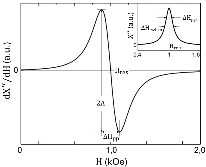
Figure 2 shows a typical FMR spectra of a ferromagnet. Depending on the type of experimental setup, the signal that you measure can be a first derivative of χ” with respect to Hwhen field modulation is used. When pulse modulation is used, the signal is measured directly as a Lorentzian function, as shown in the inset. Chapter 2 will explain the experimental setup in more detail.
When analyzing the measured signal as shown in Figure 2, a few characteristics can be extracted by fitting the curve.
- The peak-to-peak value (ΔHpp),
- The strength of the signal (amplitude A),
- The resonance field strength (Hres)
Conversely, when using pulse modulation, we observe a signal as shown in the top right inset of Figure 2; a Lorentzian function. It makes less sense to talk about peak-to-peak values, but rather about the Full Width at Half Maximum (FWHM), ΔHFWHM. As shown, this is not the same as the peak-to-peak value. The relation between the two is as follows:
\[\Delta H_\textrm{FWHM} = \sqrt{3}\Delta H_\textrm{pp}\].
The goal is to measure these parameters at multiple frequencies, and plot them as shown in Figure 3. Fitting your obtained results with the Kittel formula allows you to extract useful characters of your sample, such as the saturation magnetization (Ms), the damping (α), and more.
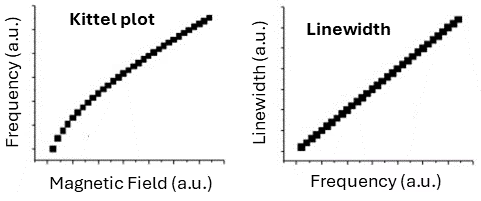
To derive the Kittel formula, we need to simplify Eq. 1 further. We know that the damping is typically in the order of 10-3 to 10-5, hence we can neglect it completely (α << 1). This gives the equation: \[(\omega_\textrm{res}/\gamma)^2 = AB\]
Replacing A and B, and neglecting the anisotropy constants, (smaller then the field at resonance), we obtain the Kittel formula. Below I show the equation for both the CGS unit system and the SI unit system [3].
Gaussian (CGS) unit system
\[f = \frac{\gamma}{2\pi} \sqrt{H_\textrm{res}(H_\textrm{res}+4\pi M_\textrm{res})}\]
With Hres and Mres in Oersted. Side note; if the surface anisotropy is neglected, Mres = Ms.
Lastly, we can extract the damping with the following equation:
\[\Delta H_\textrm{pp} =\Delta H_\textrm{0}+\frac{4\pi}{\sqrt{3}\gamma}f\alpha\]
where ΔH0 is the inhomogeneous linewidth broadening, more on this later on.
As mentioned before, in some literature you will find that they use the full width at half maximum (FWHM) instead of peak-to-peak values. This mainly depends if you are measuring the actual absorption or its derivative. Hence you might see the equation without the √3 as well [2, 3].
SI unit system
In modern scientific papers, it is common to use the “Système International d’Unités,” or International System of Units (SI). The use of units is generally clear, but confusion can still arise between B, H and μ0H . In simplified cases, it is often stated that B = μ0H. Below is such an example, of the Kittel equation expressed in SI units:
\[f = \frac{\gamma \mu_0}{2\pi} \sqrt{H_\textrm{res}(H_\textrm{res}+M_\textrm{res})}\]
With μ0Hres and μ0Mres in Tesla.
2. Experimental setup
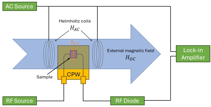
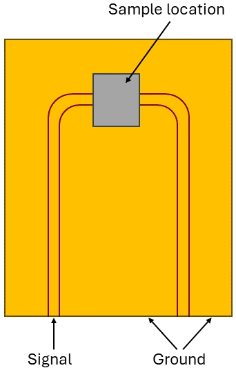
The most important parts of a broadband FMR spectroscopy measurement setup are shown in Figure 1, 4 and Figure 5. The role of the coplanar waveguide (CPW) is to transmit a microwave signal from an RF source at a broad range of frequencies (normally ranging from 2 GHz to 40 GHz). Near the CPW, the magnetic component of the micowave source, hrf, can excite the magnetic sample, at the appropriate magnetic field (HDC) and frequency. As hrf does not extend far from the CPW, the sample should be placed with the magnetic film side down. It is important that the magnetic film has a thin insulating layer, to not short the CPW.
Most FMR measurements are performed using a fixed frequency and sweep the magnetic field (HDC). When the field passes through the resonance condition, the magnetization in the material will begin to precess, and therefore absorb energy from the CPW. This drop in DC voltage is being measured at the RF diode.
2.1 Lock-in amplifier
To enhance the signal-to-noise ratio, a lock-in amplifier is often employed. This device uses a modulating magnetic field (HAC) at a known frequency. To generate this modulated magnetic field, a set of Helmholtz coils powered by an AC source is utilized. The amplitude of the AC magnetic field is approximately 1 Oe and is superimposed on the larger HDC field.
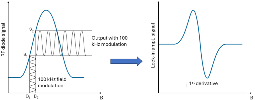
Figure 6 illustrates the concept of the lock-in amplifier. During the sweep of the large HDC field, a small AC magnetic field with a fixed frequency of 100 kHz modulates the signal. Under resonance conditions, this small modulating field produces a significant signal during the rising and falling portions of the resonance absorption signal. When the RF diode signal is flat (at its peak and outside of resonance under ideal conditions), the lock-in amplifier signal is also zero. This method effectively generates a derivative of the absorption signal.
3. Inverse spin Hall effect (ISHE)
When a ferromagnet/non-magnetic bilayer sample gets placed in an FMR, at resonance, a flow of spins from the ferromagnet will enter the non-magnetic layer due to a phenomenon called spin pumping. Especially in heavy-metal layers with large spin orbit interaction, will this spin current be significant. Through the inverse spin Hall effect will this spin current be converted into a charge current, which we can measure as a transverse DC voltage.
This effect can be measured on the FMR setup as described above, however, measuring the ISHE on the metallic surface while it is laying flat on the CPW can be difficult. That is why, most spin pumping measurements are done on a resonance cavity FMR setup.
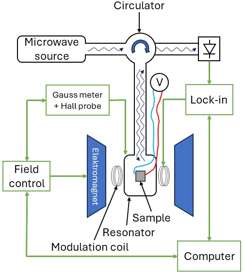
A resonance cavity is a enclosed space, that sustains electromagnetic standing waves or electromagnetic oscillations. The cavity is coupled with an external circuit that provides the energy to the system with the microwave source. On the other hand, the excited cavity provides the energy to the sample. The basic structure of the resonance cavity is shown in Figure 7. The coupling of the cavity with the sample can be best understood by an LCR equivalent circuit, hence resonance cavities are often described with a Q-factor that explains how well it couples.
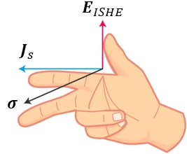
To measure the inverse spin Hall effect voltage on the metallic layer, both ends need to be connected to either a (nano) voltage meter, or another lock-in amplifier. The method to connect the surface to an external wire is sometimes challenging; I’ve personally used a technique called ball bonding, to connect the sample to a conductive pad (which is than connected to the outside measurement device). Another important topic of discussion, is how to place your sample and which sides to connect. Preferably, if you have a rectangular shape, you want to measure the voltage along the longer side, as the voltage scales with the width. The induced electric field EISHE is transverse to the spin current Js and σ; and is therefore given by [6]:
\[\textbf{E}_\textrm{ISHE} \propto\textbf{J}_\textrm{s} \times \sigma\]
4. References
[1] H. Kyu Lee, Magnetic Anisotropy, Damping and Interfacial Spin Transport in Pt/LSMO Bilayers, Master Thesis, University of California, Irvine (2017).
[2] J. T. van Galen, Building a Ferromagnetic Resonance Setup, Master Thesis, Eindhoven, University of Technology (2017).
[3] Quantum Design, Application Note 1087-201, Introduction to: Broadband FMR spectroscopy (2017), Available online: https://qdusa.com/siteDocs/appNotes/1087-201.pdf.
[4] http://www.sampleinst.com/index/Page/index.html?cate=48
[5] C.-K. Lo, ‘Instrumentation for Ferromagnetic Resonance Spectrometer’, Ferromagnetic Resonance – Theory and Applications. InTech, Jul. 31, 2013. doi: 10.5772/56069.
[6] K. Ando, S. Takahashi, J. Ieda, Inverse spin-Hall effect induced by spin pumping in metallic system, J. of Appl. Physics, vol. 109, 10 (2011).
Florius
Hi, welcome to my website. I am writing about my previous studies, work & research related topics and other interests. I hope you enjoy reading it and that you learned something new.
More Posts


Comments
Simply a smiling visitant here to share the love (:, btw outstanding pattern.