
For most electrical systems, we deal with either direct current (DC) or alternating current (AC). DC is usually well understood — it feels intuitive: there’s a clear voltage drop across a resistor, and the current can be found simply by dividing voltage by resistance. AC, on the other hand, often feels more mysterious. I frequently hear questions like, “How can AC power a motor or light a lamp if the voltage and current are constantly oscillating back and forth?” In my previous post on AC motors, I already explored how these devices work.
Table of Contents
In this article, I’ll focus on how DC and AC voltage actually transfers energy, even though the average current over a full cycle is zero. Using equations, I’ll show that the instantaneous power remains positive throughout each cycle. Then, I’ll dig a little deeper into the physics, revealing that the true mechanism of energy transport in AC circuits is quite different from what most people imagine and it might surprise you.
Why AC Power Still Heats Your Bulb
An ideal AC voltage behaves like a sine wave. However, the average of a pure sine wave over a cycle is zero, and you might think that it is useless. However, when you hook it up to a heater, or an (oldschool) lamp, the electrons don’t care if the voltage is positive or negative. They just care about how much energy they can put into the system, and that depends on the square of the votlage as we will see later on.

Instead of calculating with squared voltages, someone had the idea to square the sine wave, to have everything positive, take the average of that (as energy builds up over time), and take the square root to get it back into volts. This is Root Mean Square (RMS). That way, when you say 230 VRMS in Europe, you are actually saying that the AC supply will deliver the same heating power as 230 VDC would.
The Idea Behind RMS Voltage
An ideal AC voltage behaves like a sine wave. However, the average of a pure sine wave over a cycle is zero, and you might think that it is useless. However, when you hook it up to a heater, or an (oldschool) lamp, the electrons don’t care if the voltage is positive or negative. They just care about how much energy they can put into the system, and that depends on the square of the votlage as we will see later on.
Instead of calculating with squared voltages, someone had the idea to square the sine wave, to have everything positive, take the average of that (as energy builds up over time), and take the square root to get it back into volts. This is Root Mean Square (RMS). That way, when you say 230 VRMS in Europe, you are actually saying that the AC supply will deliver the same heating power as 230 VDC would.
To understand the last sentence better and to relate VRMS to VDC we will take a look at some maths. Take a simple AC sine wave voltage:
\[v(t)= V_{peak}\cdot\text{sin}(\omega t)\]
When you hook it up to a light bulb, we can model it as a resistor R, so that the current is:
\[i(t) = \frac{v(t)}{R}=\frac{V_{peak}}{R}\cdot\text{sin}(\omega t)\]
Now the instantaneous power (the actual joules being dumped per second) is
\[p(t)=v(t)\cdot i(t) = \frac{V^2_{peak}}{R}\cdot \text{sin}(\omega t)\]
Here we can see that the power really depends on sin2, which is always positive. That is why the filament (or resistor) always gets heated, no matter the direction of the voltage. To link DC voltage and RMS voltage, we need to look at the average power over time, this is done by:
\[P_{avg} = \frac{1}{T}\int_0^T\text{sin}^2(\omega t) dt\]
where T is one period. If we plug the variable p(t) in, we get:
\[P_{avg}=\frac{V^2_{peak}}{R}\cdot\frac{1}{T}\int^T_0\text{sin}^2(\omega t) dt\]
We know that the average of sin2 over a full cycle is exactly 1/2, thus:
\[P_{avg}=\frac{V^2_{peak}}{2R}\]
Now if we compare this to DC. With a constant DC voltage VDC, the power would be:
\[P=\frac{V^2_{DC}}{R}\]
if we want AC to give the same heating as DC, we set them equal:
\[\frac{V^2_{DC}}{R}=\frac{V_{peak}^2}{2R}\]
This can be written as :
\[V_{DC} = \frac{V_{peak}}{\sqrt{2}}\]
This is exactly the RMS value. When talking about Europe, we normally say it has VAC = VRMS = 230 V, which actually means 325 Vpeak in the wires. In theory you could use 230 VDC on a lightbulb, and it would shine with the same brightness and same power draw as RMS 230 VAC. However, I wouldn’t recommend doing it, as there are other issues. Your house wiring and circuit breakers are designed with AC in mind. I can also imagine that DC can create a lot of sparks, that are being surprised by AC, as it crosses zero 100 times a second (50 Hz).
With a plain resistor, RMS voltages translate cleanly into power, as voltage and current are in phase. When we add coils or capacitors, it is no longer this easy. The RMS of voltage and current is still defined the same way, but what changes is how much of that power actually is used as real power. I hope to come back to this at a later stage to talk about apparent power, reactive power and the power factor.
Where the Power Really Flows
You may think that the electrons fly through the copper wire, from the energy plant to your lightbulb and back again, 50 times a second. This is what most people think, but its wrong. Electrons have a thermal motion (105 m/s), but it is random. When an electric field is applied, they pick a tiny net velocity in the direction opposite to the field, this is called drift velocity. For household currents in copper wires, the drift velocity is small, perhaps in the range of millimeters per second or less. In AC, the electric field reverses 50 times a second, so electrons just oscillate back and forth with the field. This is called the drude model, and is better explained in one of my previous articles.
The real energy isn’t being carried by the electrons itself, but by the electromagnetic field around the wire. That field propagates at a significant fraction of the speed of light along the wires. When the field reaches the filament (or resistor), it excerts a force on the local electrons there, oscillating them back and forth. They collide with the filament atoms, which is the source of heat and light.
In the Feynman lectures [1] we read:
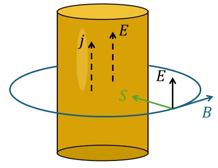
We ask what happens in a piece of resistance wire when it is carrying a current. Since the wire has resistance, there is an electric field along it, driving the current. Because there is a potential
drop along the wire, there is also an electric field just outside the wire, parallel to the surface Fig. 27-5. There is, in addition, a magnetic field which goes around the wire because of the current. The E and B are at right angles; therefore there is a Poynting vector directed radially inward, as shown in the figure. There is a flow of energy into the wire all around. It is of course, equal to the energy being lost in the wire in the form of heat. So our ‘‘crazy’’ theory says that the electrons are getting their energy to generate heat because of the energy flowing into the wire from the field outside. Intuition would seem to tell us that the electrons get their energy from being pushed along the wire, so the energy should be flowing down or up along the wire. But the theory says that the electrons are really being pushed by an electric field, which has come from some charges very far away, and that the electrons get their energy for generating heat from these fields. The energy somehow flows from the distant charges into a wide area of space and then inward to the wire.
Feynman used to Poynting vector in the following way. The flow of the electromagnetic fields around the circuit is described by the Poynting vector:
\[\vec{S} = \frac{1}{\mu_0}\vec{E}\times\vec{B}\]
where E the electric field, and B is the magnetic field, created by the current. Their cross product gives the Poynting vector (S), which points in the direction of real energy transfer. An example is given in Figure 3, where the field is along the wire, and the magnetic field, created by the current, goes in concentric circles around the wire. In this case, the Poynting vector S would be directed into the wire. In the sections below, I will use Sommerfeld’s model [2] for electric current to explain how energy flows in an electric circuit. Most of the information here is taken from [3] as inspiration.
Open Circuit: No Flow
When a battery isn’t connected to anything, its basically a static dipole. You’ve got:
- One terminal at a higher potential (positive side),
- The other at a lower potential (negative plate),
- A chemical mechanism that keeps the charges separate.
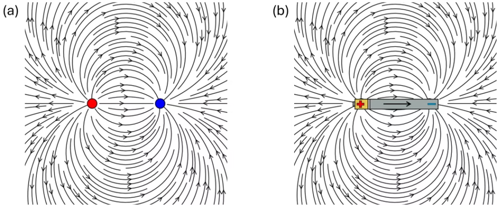
This way, you end up with an electric field in the space around it, just like the field of a physical dipole (pointing from + to – in the external region). Inside the battery its a bit more complicated, as the chemical charges work against the electrostatic field to maintain the separation. As long as the battery is disconnected, no continuous flow of charge is present, so no current. And without current, there is no magnetic field. We can see this from Maxwell’s equations, the relevant part is:
\[\nabla\times\vec{B} = \mu_0\vec{J}+\mu_0\varepsilon_0\frac{\partial\vec{E}}{\partial t}\]
That means magnetic fields are generated by current J (moving charges), or changing electric field. And if the battery is disconnected, neither one of them is present, so the magnetic field is zero everwhere. That means that Poynting vector S is also zero and there is no real energy transfer.
DC Circuit: Steady Fields
We can now start discussing the energy transfer in a simple closed circuit, beginning with a description of the electric field along a homogeneous wire of uniform cross section, which is connected to the terminals of a battery.
Inside the wire, the electric field is directed along the wire and has a constant magnitude in steady state. This uniform internal field drives the motion of conduction electrons and is sustained by the steady gradient of surface charge along the wire.
At and near the surface, the electric field can be viewed as having two components. The normal component En (pointing outward or inward, depending on the local surface charge), and a tangential component Eτ, parallel to the wire, aligned with the current density j. The normal component varies along the wire, reflecting the changing surface charge, while Eτ remains constant just inside and outside the conductor, satisfying boundary conditions.
Inside the battery, electrochemical charge separation produces an internal current opposite to that in the external circuit. This internal current closes the loop and maintains the steady flow of charge through the entire circuit.
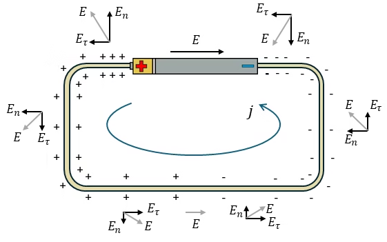
In the idealized case of a perfect conductor (zero resistivity), the Sommerfeld solution shows that the electric field outside the wire is purely normal to its surface (Eτ = 0). Because current can flow without resistance, there is no need for a tangential electric field: electrons move freely, and no surface-charge gradient develops along the wire. This situation is illustrated in Figure 6 (a), where the normal component En dominates around the perfectly conducting loop.
When a resistor is introduced, however, the situation changes. To maintain a steady current through the resistor, an electric field must exist inside it, directed from the positive side toward the negative. Since the field along the ideal wires is perpendicular to their surface and effectively zero inside, the field near the junctions must rotate to connect these two regions. This transition happens through a continuous bending of the electric field lines, guided by surface charges at the interfaces, as indicated in Figure 6 (a) by the bending of the field lines and the appearance of a tangential component Eτ.
In the region of the resistor where the surface charge transitions from positive to negative, there is a neutral point where the charge density passes through zero. As this happens, the electric field outside the conductor gradually changes direction, from pointing outward near the positively charged side to inward near the negatively charged side. Instead of an abrupt jump, the field bends smoothly, reorienting from the wire’s surface into the resistor body.
This continuous change is illustrated in Figure 6 (b), where the electric field lines form gentle arcs that connect the field just outside the wires to the nearly uniform field inside the resistor, showing how the direction of E reverses smoothly across the resistor region.
Overall, the electric field points from the positive to the negative terminal throughout the circuit—inside the battery, the wires, and the resistor. Outside the conductors, E varies smoothly in both magnitude and direction, completing an overall 180° rotation around the outer region of the loop, consistent with the field geometry seen in Figure 6 (b).
Now that the electric fields are clear, we can examine how the magnetic fields are created.
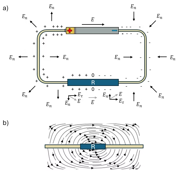
According to the Ampère-Maxwell law, the magnetic field lines curl around the current, forming concentric circles around each wire. These circles follow the right-hand rule.
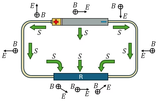
In Figure 7, the magnetic field is shown only outside the circuit (represented by ⊕), indicating that it points into the page. With both the directions of the electric field and magnetic field established, we can now describe how energy is transported through the circuit using the Poynting vector S, shown by the green arrows.
Inside the battery, S points outward, illustrating that electromagnetic energy is delivered from the chemical source into the electromagnetic field surrounding the circuit. Along the wires, S runs approximately parallel to their surfaces, directed away from the battery on both sides and toward the resistor.
As the energy approaches the resistor, the electric field outside it rotates due to the local surface-charge distribution, and S turns correspondingly. At the midpoint of the resistor, where the surface charge changes sign, S points straight into the resistor, indicating that electromagnetic energy is absorbed and converted into thermal energy (heat).
The overall result is that the electromagnetic energy flux always flows from the battery to the resistor and never the opposite direction, exactly as we expect for a dissipative DC circuit.
AC Circuit: Oscillating Fields
To explain AC circuits, it is good to start explaining electromagnetic waves. In a free-space propagating electromagnetic wave, the two fields are in phase:
\[\vec{E}(z,t) =E_0\text{cos}(kz-\omega t)\hat{x}\]
\[\vec{B}(z,t) =B_0\text{cos}(kz-\omega t)\hat{y}\]
where E0 and B0 are the amplitudes, k is the wavevector and ω is the angle frequency. Both waves oscillate in phase; if E is at its maximum, so is B. This can be seen in Figure 8, where both fields are plotted.
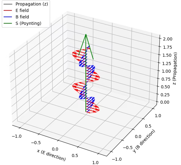
The Poynting vector can be calculated in the following way:
\[\vec{S}(z,t) = \frac{E_0B_0}{\mu_0}\text{cos}^2(kz-\omega t)\hat{z}\]
where the direction of S is constant and directed in the positive z axis. The amplitude oscillates between 0 its maximum, because cos2(θ) is always positive (between 0 and 1). This means that the energy flows continuously forward, while the strength of that flow oscillates rhythmically over time. On average, this results in a constant light intensity.
Returning to our circuit, if we apply an AC source, the Poynting vector will likewise remain directed from the source toward the load, indicating that energy continues to flow in the same overall direction throughout each cycle.
References
[1] R. P. Feynman, R. B. Leighton, and M. Sands, The Feynman Lectures on Physics, Vol. II: Mainly Electromagnetism and Matter, New Millennium ed. New York, NY, USA: Basic Books, 2011, pp. 27–28.
[2] A. Sommerfeld, Electrodynamics, vol. 3 of Lectures on Theoretical Physics, trans. E. G. Ramberg. New York, NY, USA: Academic Press, 1952, pp. 125–130.
[3] I. Galili and E. Goihbarg, “Energy transfer in electrical circuits: A qualitative account,” American Journal of Physics, vol. 73, no. 2, pp. 141–144, Feb. 2005, doi: 10.1119/1.1819932.
Florius
Hi, welcome to my website. I am writing about my previous studies, work & research related topics and other interests. I hope you enjoy reading it and that you learned something new.
More Posts