


Over the past few months, I have been looking at several interesting topics, and I forgot to pay much focus on this blog. One of those projects is building my own neural-network-based AI. The project is now nearly complete, but I wanted to document what I have learned before I start forgetting the small details.
During this process, I got fascinated by the connections between seemingly different subjects, such as PID control systems, feedback loops, error correction, logic gates, and neural networks. Simple Boolean functions such as AND, OR, and XOR have long been used to demonstrate what neural networks can and cannot learn. These small examples can explain the fundamentals that are used for larger AI systems: weigths, hidden layers, training and prediction.
This post is the first in a new series in which I will go deeper into those ideas, starting with how neural networks can learn the behaviour of logic gates. Enjoy reading!
Table of Contents
The connection between logic and neural networks goes back to 1943, when Warren McCulloch and Walter Pitts introduced a simplified mathematical model of a biological neuron [1]. In their paper, a neuron either fires or remains inactive, depending on whether its combined inputs cross a threshold. Networks of these neurons could reproduce logical operations such as AND and OR. Real biological neurons are far more complicated, but this provided an important bridge between neuroscience, logic, and computation.
In 1957, psychologist Frank Rosenblatt developed the perceptron; an artificial neuron that could learn by adjusting its connections (weights). A demonstration followed in 1958 on an IBM 704, a room-sized computer that learned to distinguish cards marked on the left from cards marked on the right [2]. Rosenblatt later built the Mark I Perceptron, a dedicated machine for recognizing simple visual patterns.
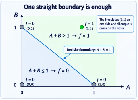
The perceptron was promising, but it had an important limitation. In their 1969 book Perceptrons, Marvin Minsky and Seymour Papert mathematically examined what these systems could and could not compute [3]. A single-layer perceptron can learn only linearly separable patterns, which are patterns whose output classes can be divided by a single straight decision boundary.
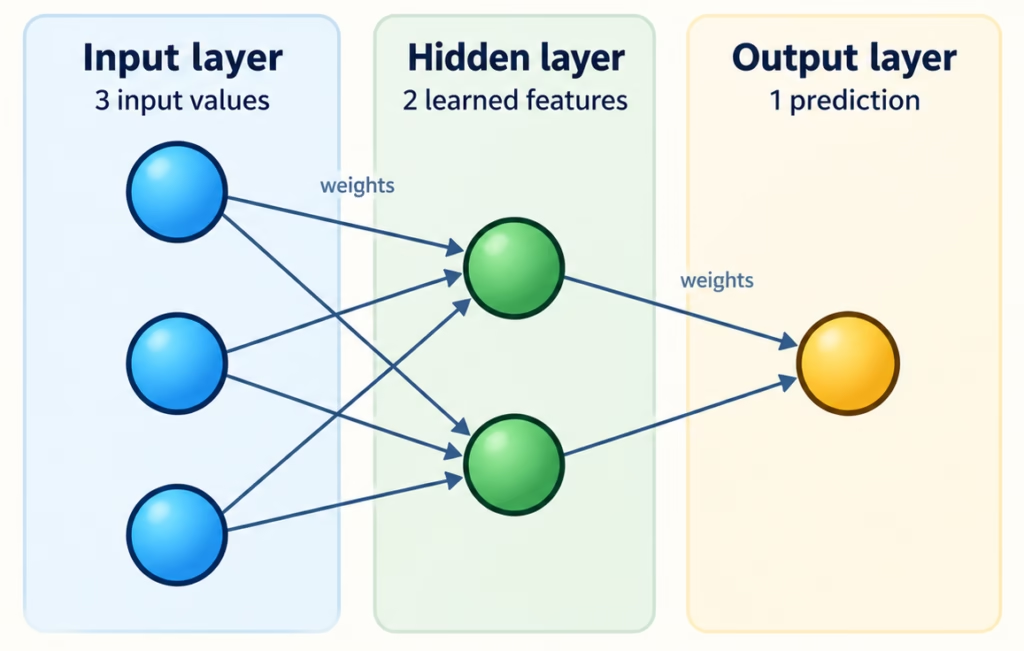
AND and OR satisfy this requirement, but XOR does not. Although a network with a hidden layer can represent XOR, researchers at the time lacked an effective general method for training such multilayer networks. This small logic problem therefore provides an ideal path through the foundations of neural networks: beginning with a single perceptron, discovering its limitations, adding a hidden layer, and finally learning its weights through backpropagation.
Logic Gates
The perceptron is just an algorithm that maps its input \(x\) to an output value \(f(x)\), similar to logic gates.
\(f(x) =
\begin{cases}
1 & \text{if } (w \cdot x + b) > 0 \\
0 & \text{otherwise}
\end{cases}
\)
Here \(w\) are the real-valued weights, \(w \cdot x\) is the dot product \(\sum_{i=1}^{n} w_i \cdot x_i\), \(n\) is the number of inputs to the perceptron,
\(b\) is a value that shifts the decision boundary away from the origin and does not depend on any input value.
A single perceptron can solve linearly separable patterns, and this can be shown by either an AND gate, or an OR gate. In the following sub-chapters I give a brief overview of some of the main logic gates. More in-depth explanations, such as how they reached these values can be found here [4].
AND Gate
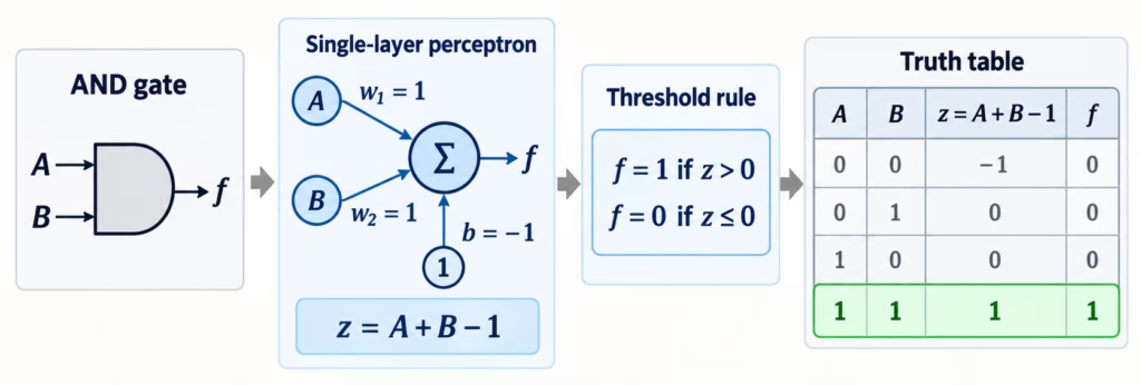
The AND gate demonstrates how a perceptron makes a binary decision, either 0 or 1. Each input is multiplied by a weight \(w_i\), after which the bias shifts the decision further. With \(w_1= w_2 = 1\), and \(b = -1\), the sum is
\[
z=A+B-1
\]
The output becomes 1 only when both inputs are 1. This works because the four input combinations can be separated by one linear decision boundary.
OR Gate
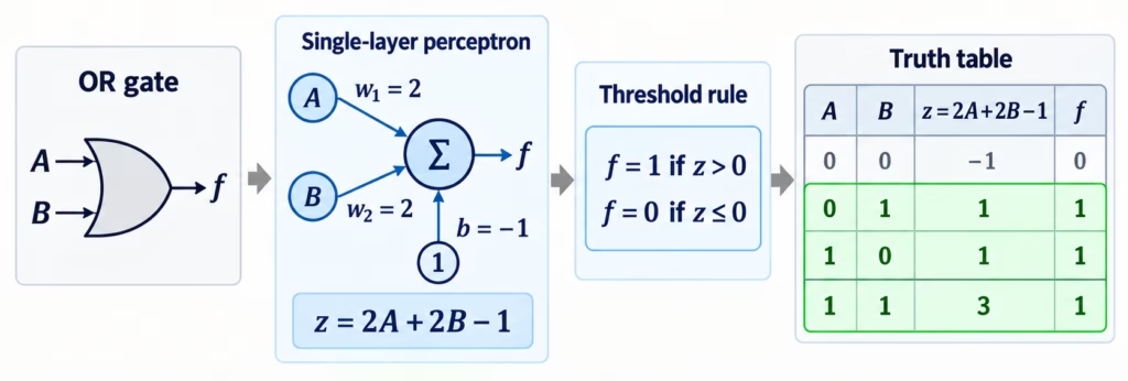
The OR gate can be modelled in the same way, but with a threshold that is exceeded as soon as either input is active. Using \(w_1=w_2=2\) and \(b=-1\), the weighted sum becomes
\[
z=2A+2B-1.
\]
Only \(A=B=0\) produces a non-positive result. Every other combination produces an output of 1. Like AND, OR is linearly separable and can therefore be represented by a single perceptron.
XOR Gate
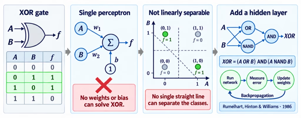
An XOR gate produces an output of 1 when exactly one of its inputs, \(A\) or \(B\), is 1. Unlike AND and OR, XOR cannot be done using a single perceptron. No matter what the values is chosen for the weights and bias \(b\), no single straight decision boundary can separate the input combinations that produce 1 from those that produce 0. Therefore XOR is not linearly separable.
Electronic logic provides a clue to the solution. An XOR gate can be constructed using OR, NAND, and AND gates:
\[
\mathrm{XOR}(A,B)
=
(A\ \mathrm{OR}\ B)
\ \mathrm{AND}\
(A\ \mathrm{NAND}\ B).
\]The OR and NAND operations can be viewed as a hidden processing layer, whose outputs are passed to the final AND operation. Similarly, a neural network needs at least one hidden layer to model XOR.
So far, we have chosen the weights ourselves. In a neural network, however, these weights can be learned from examples. In their influential 1986 paper, David Rumelhart, Geoffrey Hinton, and Ronald Williams described how backpropagation could be used to train multilayer networks. The network first makes a prediction and measures its error. That error is then propagated backward through the network to determine how each weight contributed to it. The weights are adjusted slightly, reducing the error over repeated training steps.
To solve XOR: Hidden layer & Backpropagation
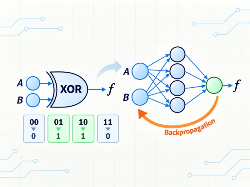
To solve XOR, we replace the single perceptron with a \(2 \rightarrow 4 \rightarrow 1\) neural network. The two input values are passed to four neurons in a hidden layer, whose outputs are then combined by one output neuron. As a disclaimer, an XOR can also be solved with only two, but it’s more reliable with four [5].
Each hidden neuron has its own weights and bias (as shown before), which determine how strongly it responds to \(A\), \(B\), or particular combinations of the two. The weights are initialized with small random values so that the neurons start differently and can develop their own specialities. If they all started identically, they would produce the same outputs and receive the same updates, making them redundant copies of one another, and you end up with basically 1 hidden neuron.
The neurons use the sigmoid activation function to introduce nonlinearity. Without a nonlinear activation function, stacking multiple layers would still be equivalent to a single linear transformation and could not solve XOR.
During a forward pass (steps 2 and 3 in Figure 6), the network calculates a prediction for each row of the XOR truth table and compares it with the expected output to measure the error. Backpropagation (step 4) then sends information about that error backward through the network, adjusting each weight and bias in the direction that reduces the error (step 5). By repeating this process over many training epochs, the hidden neurons learn different features and the network gradually learns the XOR pattern (step 6).
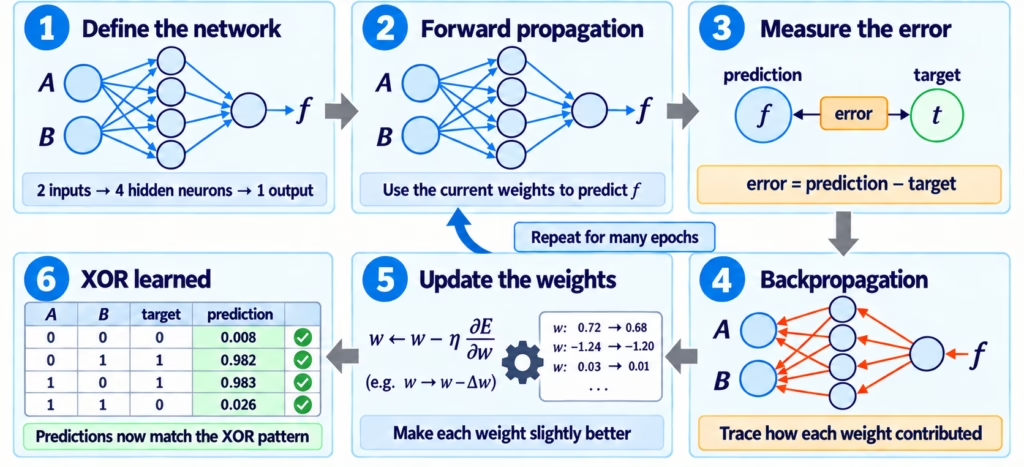
Step 4: Backpropagation
During the forward pass, information travels from input to the prediction:
\[ A,B \rightarrow \text{hidden layer} \rightarrow \text{prediction} \]
After comparing the prediction with the target, the network knows how wrong the final output is, but it does not yet know which connections in the network caused that error.
Backpropagation sends this error information through the network in the opposite direction:
\[ \text{error} \rightarrow \text{output neuron} \rightarrow \text{hidden neurons} \]
For every weight, it calculates a gradient:
\[ \frac{\partial E}{\partial w} \]
This value answers two questions:
- Did this weight increase or decrease the error?
- How strongly did this weight affect the error?
A positive gradient means reducing the weight should reduce the error. A negative gradient means increasing it should reduce the error. And a gradient close to zero means the weight had little effect at all.
In the step 4 of backpropagation, it only calculates and records the corrections required for every weight without changing anything.
Step 5: Weight update: apply the calculated corrections
After the gradients have been calculated, the optimizer applies them:
\[ w_{\text{new}} = w_{\text{old}} – \eta\frac{\partial E}{\partial w} \]
Here:
- \(w_{\text{old}}\) is the current weight.
- \(\frac{\partial E}{\partial w}\) is the correction calculated by backpropagation.
- \(\eta\) is the learning rate, which controls the size of the adjustment (which I set to 1).
- \(w_{\text{new}}\) is the adjusted weight.
The two stages are kept separate, because changing one weight immediately could affect the calculations for the remaining weights, and that is not something we want. We need to change them all at once every time we go round.
From Training to a Trained Model
During one epoch, the network processes every row of the XOR truth table once. For each example, it performs a forward pass, measures the error, propagates that error backward, and updates its weights and biases. The first epoch produces poor predictions because the parameters were initialized randomly.
The network then repeats the same process for many epochs. Each pass makes small corrections, gradually reducing the prediction error. It is not memorizing Python instructions or adding new neurons; it is only adjusting the numerical values stored in its weights and biases.
After training, the network no longer needs backpropagation to solve XOR. The 17 learned parameters can be saved to a file:
- \((2\times 4=8)\ \text{Input} \rightarrow \text{hidden weights}\)
- \((4)\ \text{Hidden biases}\)
- \((4)\ \text{Hidden} \rightarrow \text{output weights}\)
- \( (1)\ \text{Output bias}\).
input_weights = [
    [ 3.557573, -2.605144, -6.481529, -6.361972],  # A → H1–H4
    [-6.523345, -2.513968,  2.289971, -6.343151],  # B → H1–H4
]

hidden_biases = [
    -1.083835,
    -0.874269,
     0.192241,
     1.988638,
]

output_weights = [
     8.827278,
    -1.482470,
     8.786671,
    -8.457829,
]

output_bias = -3.944379
With this set of values, it has now learned a mapping:
\((A,B)\longrightarrow f(A,B)\)
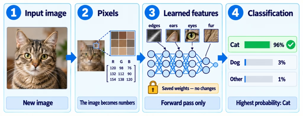
However, the XOR example only has four possible inputs (0,0), (0,1), (1,0), (1,1), and all four inputs are included in the training. There are no unseen XOR combinations, as there are none, therefore this doesn’t seem like the best example. But the same principle scales to millions of possible inputs. Such as a network that trains on images and then uses its learned weights to classify images it has never seen before.
References
[1] W. S. McCulloch and W. Pitts, “A logical calculus of the ideas immanent in nervous activity,” Bulletin of Mathematical Biophysics, vol. 5, pp. 115–133, Dec. 1943, doi: 10.1007/BF02478259.
[2] M. Lefkowitz, “Professor’s perceptron paved the way for AI—60 years too soon,” Cornell Chronicle, Sep. 25, 2019. [Online]. Available: https://news.cornell.edu/stories/2019/09/professors-perceptron-paved-way-ai-60-years-too-soon. [Accessed: Sep. 17, 2026].
[3] M. Minsky and S. A. Papert, Perceptrons: An Introduction to Computational Geometry. Cambridge, MA, USA: MIT Press, 1969.
[4] P. Upadhyaya, “Neural Representation of AND/OR/NAND/XOR Logic Gates (using Perceptron Algorithm),” Jan. 2023. [Online]. Available: https://www.researchgate.net/publication/366902248_Neural_Representation_of_ANDORNANDXOR_Logic_Gates_using_Perceptron_Algorithm. [Accessed: Sep. 16, 2026].
[5] D. Yang, “Building an XOR Neural Network from Scratch: Learn from the Basics,” Medium, Aug. 3, 2024. [Online]. Available: https://medium.com/@derek246810/building-an-xor-neural-network-from-scratch-learn-from-the-basics-63a2a22495ae. [Accessed: Sep. 16, 2026].
[6] Syntax, “I Built an LLM From Scratch,” YouTube, Jul. 10, 2026. [Online]. Available: https://www.youtube.com/watch?v=YmLp8qe87A0. [Accessed: Sep. 16, 2026].

Florius
Hi, welcome to my website. I am writing about my previous studies, work & research related topics and other interests. I hope you enjoy reading it and that you learned something new.
More Posts