

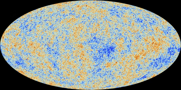
If you follow astrophysics even casually, you have likely heard of the Cosmic Microwave Background (CMB). It is the faint radiation that fills all of space in the observable universe. To the naked eye, the space between stars appears black. But with sufficiently sensitive instruments, that darkness shows a nearly uniform background glow coming from every direction. This radiation has a thermal blackbody temperature of about 2.725 K, with tiny fluctuations of only a few ten-thousandths of a kelvin. Those minute variations are not noise; they encode information about the structure and evolution of the early universe. Such a temperature map can be seen in Figure 1.
The CMB is usually presented as a full-sky temperature map, where color represents these small fluctuations (see Figure 1). At first glance such maps can feel abstract: a flat, oval image that somehow represents the entire sky. Initially, I didn’t understood how such a map covers the entire sky.
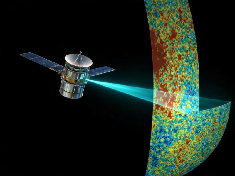
In this post, I will not go into full detail on the CMB itself, but rather try to make mapping from 3D to 2D understandable for everyone. Nonetheless I still need to briefly explain what the CMB is and how we can map it. I begin with the radiation wrapped onto a 3D sphere, emphasizing a simple but important fact: the CMB is not “out there” in one direction, but it surrounds us completely. Scanning-style animations then show how a telescope observes the sky piece by piece, and how those observations are combined and unfolded into a two-dimensional projection without losing their global context.
Cosmic Microwave Background
The cosmic microwave background is the faint thermal radiation that fills all of space. It literally is the oldest light we can observe, released when the universe was about 300,000 years old. Why it took this time, and where the light comes from is best explained here.
What is important for this article, is why is it everywhere? Because the big bang didnt happen at a single point in space, it happened everywhere at once. So that when the universe became transparant, light was emitted in all directions, from all places. The small imperfections at that time in space, is what we measure rigt now as very small temperature differences. These differences later grew (via gravity) into galaxies, and larger clusters.
Experimental Instruments
Because the temperature variations in the Cosmic Microwave Background are extremely small, measuring them requires exceptionally clean and stable instruments. Although ground-based telescopes can detect parts of the signal, the most reliable measurements come from space-based satellites. Observing from space avoids atmospheric interference and allows full-sky mapping with high precision.
Over the past four decades, three major satellite missions have been dedicated to detecting and mapping the CMB: COBE, WMAP, and Planck.
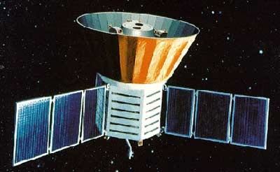
COBE (1989)
The COBE (Cosmic Background Explorer) was launched by NASA in 1989.
Its primary objective was to determine whether the CMB follows a perfect blackbody spectrum. This was successfully confirmed with extraordinary precision, a result that later earned John Mather and George Smoot the Nobel Prize in Physics.
COBE also made the first detection of temperature anisotropies in the CMB. This was a groundbreaking discovery. Before COBE, these fluctuations were only predicted theoretically. COBE provided the first direct evidence that the tiny density variations required for structure formation actually existed.
However, the satellite’s angular resolution was limited to about 7 degrees. As a result, its CMB map was relatively blurry and only revealed very large-scale structures.
WMAP (2001)
The WMAP (Wilkinson Microwave Anisotropy Probe) was launched by NASA in 2001.
Its goal was to produce high-precision maps of CMB anisotropies and to determine the fundamental cosmological parameters. WMAP achieved an angular resolution of about 0.2 degrees (approximately 13 arcminutes), a major improvement over COBE. Among its key achievements were:
- Determining the age of the universe to high precision (~13.7 billion years)
- Measuring the matter density (Ωm)
- Measuring the dark energy density (ΩΛ)
- Providing strong evidence that the universe is spatially flat
With WMAP, cosmology entered the era of precision measurement.
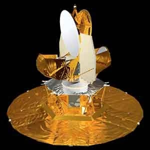
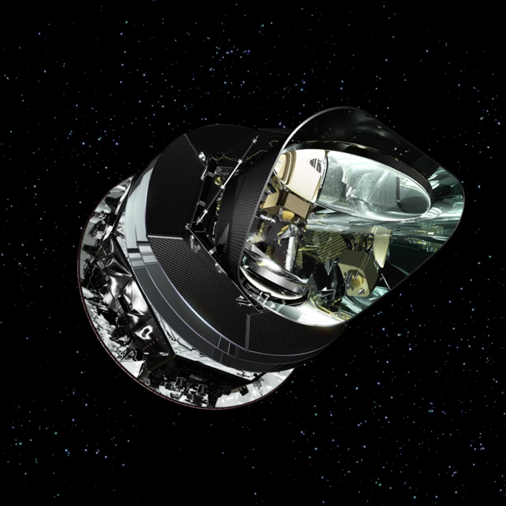
Planck (2009)
The Planck satellite was launched by the European Space Agency (ESA) in 2009. Planck represented a major technological advancement over its predecessors. It featured:
- Higher sensitivity detectors
- Improved foreground separation techniques
- Nine frequency bands for more accurate signal extraction
Its angular resolution reached about 5 arcminutes, making it the most detailed and sensitive of the three missions. Planck refined the age of the universe to approximately 13.8 billion years and placed much tighter constraints on key cosmological parameters.
Mollweide Projections in Galactic Coordinates
Now to go back to the main problem. How does the night sky gets mapped using these satellites. To answer this, we start with an analogy. Imagine the Earth as a sphere that is observed gradually, not all at once. A satellite scans the surface in narrow strips, looping around the planet and shifting slightly each time, until every latitude and longitude has been measured. Each observation is naturally tied to a point on the spherical surface. Some locations, like the North and South Poles, are special: all longitudes meet there, so each pole is always a single point, no matter how the Earth is scanned. An illustration can be seen in the figure below.
To see the entire planet at once, this spherical data has to be laid out on a flat surface. That is the role of a map projection. The Mollweide projection takes every point defined by latitude and longitude and places it inside an oval in such a way that equal areas on the Earth remain equal areas on the map. Near the equator, where the Earth’s circumference is largest, the map spreads out horizontally. Toward the poles, the available circumference shrinks, so the map compresses until all longitudes collapse into a single point at the top and bottom of the oval. In this way, the Mollweide map is simply the final step of the scan: a consistent way to unfold a fully observed sphere into one complete, area-faithful view, shown in Figure 6.
Night Sky Mapping
For the Earth, the geometry is familiar and intuitive. A satellite orbits outside the planet and looks inward. As the Earth rotates beneath it, the satellite scans the surface in narrow strips. Over time, every latitude and longitude is observed. Each measurement corresponds to a point on the Earth’s surface, and the full dataset naturally lives on the outside of a sphere.
For the Cosmic Microwave Background, the situation is inverted. There is no external vantage point. Instead, we are located inside the sphere that emits the radiation. A CMB telescope does not look toward an object at a distance; it looks outward in different directions of the sky. As the spacecraft spins and slowly changes orientation, it scans rings and arcs on the celestial sphere that surrounds the observer. After enough time, every direction has been measured.
Despite this difference in perspective, the mathematical problem is identical in both cases. Whether the data comes from scanning the Earth from the outside or scanning the sky from the inside, the result is still a complete spherical surface covered with measurements. Each data point is labeled by two angles, analogous to longitude and latitude. The poles are special in both cases: on Earth they are single points where all longitudes meet, and on the sky they are simply directions where many scan paths intersect.
Once the entire sphere has been observed, the data must be flattened into a single image. The Mollweide projection redistributes the sphere into an oval while preserving area, spreading points near the equator and compressing points near the poles until they collapse into single points at the top and bottom of the map. The Earth Mollweide and the CMB Mollweide therefore look so similar not because the underlying objects are the same, but because in both cases they represent the same thing: a complete spherical dataset, scanned in time and unfolded into a single, coherent view.
The Reality Behind the Scanning
In practice, the process is far more complex than this simplified picture suggests. CMB satellites are positioned near a gravitationally stable location known as a Lagrange point, specifically the Sun-Earth L2 point. From this location, the spacecraft remains shielded from direct sunlight and thermal interference while maintaining a stable orbit relative to both the Sun and the Earth. This stability is crucial for making extremely sensitive measurements of microkelvin-level temperature variations [5, 6, 7].
Moreover, the same patch of sky is scanned many times. Repeated observations allow scientists to:
- Reduce random noise through averaging
- Identify and remove systematic errors
- Separate foreground emissions (such as dust and synchrotron radiation) from the true CMB signal
- Improve overall sensitivity
The final map is therefore not a single scan, but the result of years of carefully calibrated measurements, statistical averaging, and sophisticated data processing.
References
[1] New Scientist, “Cosmic microwave background,” *NewScientist.com*. [Online]. Available: https://www.newscientist.com/definition/cosmic-microwave-background/. [Accessed: 12-Feb-2026].
[2] “COBE satellite image,” *space.skyrocket.de*, Gunter’s Space Page. [Online]. Available: https://space.skyrocket.de/img_sat/cobe__1.jpg. [Accessed: 12-Feb-2026].
[3] Engineering and Technology History Wiki (ETHW), “Wilkinson Microwave Anisotropy Probe (WMAP),” *ethw.org*. [Online]. Available: https://ethw.org/Wilkinson_Microwave_
Anisotropy_Probe_%28WMAP%29. [Accessed: 12-Feb-2026].
[4] European Space Agency (ESA), “Planck operations,” *ESA – Enabling & Support / Operations*, 04-Dec-2006. [Online]. Available: https://www.esa.int/Enabling_Support/Operations/Planck_operations. [Accessed: 12-Feb-2026].
[5] European Space Agency (ESA), “Planck operations,” ESA, 04-Dec-2006. [Online].
Available: https://www.esa.int/Enabling_Support/
Operations/Planck_operations. [Accessed: 12-Feb-2026].
[6] P. A. R. Ade *et al.*, “Planck 2013 results. I. Overview of products and scientific results,” *Astronomy & Astrophysics*, vol. 571, A1, Oct. 2014, doi: 10.1051/0004-6361/201321529.
[7] Berkeley Lab, “Planck – ESA Planck Surveyor Mission,” Lawrence Berkeley National Laboratory AETHER, May 2009. [Online]. Available: https://aether.lbl.gov/planck.html. [Accessed: 12-Feb-2026].
Florius
Hi, welcome to my website. I am writing about my previous studies, work & research related topics and other interests. I hope you enjoy reading it and that you learned something new.
More Posts