Updated 24 May 2024

Published 19 April 2024

The Landau-Lifshitz-Gilbert equation

1. Landau-Lifshitz equation

To model the motion of the magnetization in the time domain, the Landau-Lifshitz (LL) equation is used. It describes the evolution in time of the magnetization in a solid. The equation is as follows [1]:

$\frac{d\textbf{M}}{dt} = -\gamma_0\textbf{M}\times\textbf{H}_\textrm{eff} -\frac{\lambda}{M_s}\textbf{M}\times(\textbf{M}\times\textbf{H}_\textrm{eff})\ ,$

where $\lambda$ is a constant characteristic of the material itself, $\gamma_0 = \mu_0\gamma$ , with $\mu_0$ the permeability of free space and $\gamma$ the gyromagnetic ratio, $M_s$ is the magnetization saturation, $\textbf{H}_\textrm{eff}$ is the effective magnetic field and $\textbf{M}$ the magnetization.

In an ideal case, with only an applied magnetic field and no damping, the magnetic moment of a single spin would precess indefinitely around the effective field, this is the so-called Larmor precession, given by the term $-\gamma_0\textbf{M}\times\textbf{H}_\textrm{eff}$ as illustrated in Figure 1. This works for a single sin, but for a large ensemble of spins, the precession is influenced by the interaction with the neighbors as well. For actual materials, you have to account for the energy losses due to dissipation, Landau and Lifshitz added the second term at at the right hand side of Eq (1). that models the damping of the the system to the nearest local minimum, which is represented by the effective magnetic field, $\textbf{H}_\textrm{eff}$ . That is how the complete Landau-Lifshitz (LL) equation came to be.

2. Landau-Lifshitz-Gilbert equation

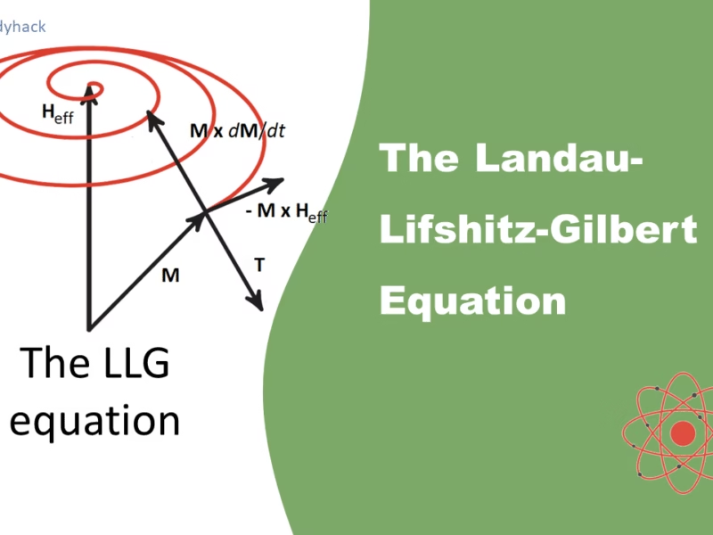
Later on, T. Gilbert [3] suggested that the term $\textbf{M}\times\frac{d\textbf{M}}{dt}$ could be used to model the damping. Figure 2 illustrates the damping of the magnetization, indicated by the inward spiraling red line. In the same figure, the torque ( $\textbf{T}$ ) is also illustrated. If this term is large enough to overcome the damping, it can flip the magnetization to $-\textbf{H}_\textrm{eff}$ . The exact mechanics of the torque will be discussed in a later section.

There is a substantial difference between the term coined by Gilbert and the one described in Eq. (1), but mathematically it can be proven to be equivalent with a normalization factor. This substitution leads to the Landau-Lifshitz-Gilbert (LLG) equation:

$\frac{d\textbf{M}}{dt} = -\gamma_0(\textbf{M}\times\textbf{H}_\textrm{eff}) + \frac{\alpha}{M_s}\textbf{M}\times\frac{d\textbf{M}}{dt} + \textbf{T}\ ,$
with $\alpha$ the Gilbert damping coefficient and the rest of the parameters are the same as above.

2.1 Proof of equavalence

Both the LL = and LLG equations are used to obtain the normalization factors and to integrate the torque and as such, the derivation to go from one to the other is shown. M. d’Aquino [4] demonstrated the equivalence between these equations. Starting with the original LLG and multiplying both sides with $\textbf{M}$ to obtain:
$\textbf{M}\times\frac{d\textbf{M}}{dt} = -\gamma_0\textbf{M}\times(\textbf{M}\times\textbf{H}_\textrm{eff}) + \textbf{M}\times\left(\frac{\alpha}{M_s}\textbf{M}\times\frac{d\textbf{M}}{dt}\right)\ .$

Making the substitution $a\times(b\times c) = b(a\cdot c) - c(a\cdot b)$ to the previous equation and by applying the following relationship $\textbf{M}\cdot\frac{d\textbf{M}}{dt} = 0$ . The last relationship can be deduced assuming that $M_s$ is onstant in time, therefore any variation in time must be a perpendicular vector to the magnetization.

$\textbf{M}\times\frac{d\textbf{M}}{dt} = -\gamma_0\textbf{M}\times(\textbf{M}\times\textbf{H}_\textrm{eff}) - \alpha M_s\frac{d\textbf{M}}{dt}\ .$
This result can be substituted back in the LLG equation, giving the following intermediate result:
$\frac{d\textbf{M}}{dt} = -\gamma_0(\textbf{M}\times\textbf{H}_\textrm{eff})-\frac{\gamma_0\alpha}{M_s}\textbf{M}\times(\textbf{M}\times\textbf{H}_\textrm{eff}) -\alpha\frac{d\textbf{M}}{dt}\ .$
By taking out the time dependency on the right hand side and moving it to the left side and grouping certain parameters together, the LLG equation can be described in the form of the Landau-Lifshitz equation in the following way:
$\frac{d\textbf{M}}{dt} = -\frac{\gamma_0}{1+\alpha^2} \textbf{M}\times\textbf{H}_\textrm{eff} - \frac{\gamma_0\alpha}{(1+\alpha^2)M_s} \textbf{M}\times(\textbf{M}\times\textbf{H}_\textrm{eff})\ .$
This form of the LLG equation is mathematically the same as the original LL equation, provided that the two parameters $\gamma_0$ and $\lambda$ in those equations are changed to the following:
$\gamma_{0}(LL) = \frac{\gamma_0}{1+\alpha^2}\ ,\ \lambda = \frac{\gamma_0\alpha}{1+\alpha^2}\ .$
Expressions are the same if the damping coefficient vanishes, Furthermore, Mallinson [5] proved that when $\lambda$ and $\alpha$ both go to infinite, then the LL equation and LLG equation give respectively:
$\frac{d\textbf{M}}{dt} \rightarrow \infty\ , \ \frac{d\textbf{M}}{dt} \rightarrow 0 \ .$
This shows that the LLG equation is more appropriate to describe the damping of the magnetization, because a large damping coefficient should have a slow motion statement, which is true for the final LLG equation and for the expression of the LL equation that considers the normalization factors. The reason to use the latter expression, is that the format of the LL equation is numerically easier to solve as there is no time dependency in the right hand side.

In conclusion, the equation that I often used, is obtained by replacing $\gamma_0$ and $\lambda$ from the original LL equation with the obtained normalization factors. This can be further rewritten to the mathematical form as programmed in the code,
$\frac{d\textbf{M}}{dt} = \frac{1}{1+\alpha^2}\left[-\textbf{M}\times\gamma_0\textbf{H}_\textrm{eff}- \frac{\alpha}{M_s}(\textbf{M}\times\textbf{M}\times\gamma_0\textbf{H}_\textrm{eff}) \right]\ ,$
where $\textbf{M}$ is the magnetization, $\gamma_0 = \mu_0\gamma$ , with $\mu_0$ the permeability of free space and $\gamma$ the gyromagnetic ratio, $M_s$ is the magnetization saturation, $\textbf{H}_\textrm{eff}$ is the effective magnetic field and $\alpha$ is the damping constant.

3. Temperature dependancy

The system described up to this point, is all purely for fictional zero degree temperatures. Non-zero temperatures would give a jiggle on the motion of the precession, effecting it ever so lightly. With high enough temperature, it can even flip the magnetization. This is one of the reasons why most of the lab work on these type of materials is done at low temperature, to keep this fluctuation to a minimum. There are many different methods to include the temperature fluctuation, such as Monte Carlo simulations, or just by adding an additional term to the LLG equation that takes this into account. For this I’d like to refer to the Master thesis of D. Schürhoff, Atomistic Spin Dynamics with Real Time Control of Simulation Parameters and Visualization (2016). It is definitely a pleasure to read such well written and informational thesis. With this, it completes the discussion of the LLG equation, its terms and their effect on a single spin.

4. References

[1] L. Landau and E. Lifshitz, “On the theory of magnetic permeability in ferromagnetic bodies.” Phys. Z. Sowjetunio, vol. 8, pp. 153-169, 1935.

[2] G.P. Muller, “Exploration of skyrmion energy landscapes,” M.S. Thesis, RWTH Aachen and FZ Julich, Germany, 2015.

[3] T. Gilbert, “A lagrandian formulation of the gyromagnetic equation of the magnetization field.” Phys Rev, vol. 100, pp. 1243, 1955.

[4] M. d’Aquino, “NONLINEAR MAGNETIZATION DYNAMICS IN THIN-FILMS AND NANOPARTICLES.” PhD Thesis, Universita degli studi di Napoli “Federico II”, Italy, 2004.

[5] J.C. Mallinson, “On damped gyromagnetic precession.” IEEE Transactions on Magnetics, vol 23, pp. 2003, 1987.

Post Views: 115

0 0 votes

Article Rating

0 Comments

Oldest

Newest Most Voted

Inline Feedbacks

View all comments