Updated 19 April 2024

Published 7 January 2024

PID tuning methods

Rule-based PID tuning methods asssume that there is a system response that can be put into an easy mathematical description. The characteristics of this response can be derived from experiments by either putting a step response on an open loop, or by tuning a closed loop system in a certain way. Note that the tuning methods described here are very sensitive to any discrepancies with respect to the assumed process (in this case a First Order Plus Dead Time, FOPDT). Deviations to the time delay will greatly degrade the PID performance.

The important PID parameters of the general PID control algorithm are presented here:

$u(t) = K_P \left( e(t) + \frac{1}{T_I} \int_{0}^{t} e(t) dt + T_D \frac{e(t)}{dt} \right)$

where

$u(t)$ = Controller output
$K_P$ = Proportional Gain
$T_I$ = Integral time
$T_D$ = Derivative time
$e(t)$ = error between setpoint and process value.

1. Heuristic tuning

This is basically the trial-and-error method. With enough experience of PID parameters, you can roughly estimate the initial guess. Especially with just a proportional controllers, you might want to give this method a try. With existing systems, you might want to tweak the parameters slightly.

In the following table I show the effects of what happens when you increase a parameter independently.

Parameter	Rise Time	Overshoot	Settling time	Steady-state error	Stability
$K_P$	Decrease	Increase	Small change	Decrease	Degrade
$K_I$	Eliminate	Increase	Increase	Eliminate	Degrade
$K_D$	Minor change	Decrease	Decrease	No effect in theory	improve if increase is small

2. Ziegler-Nichols closed-loop tuning method

The Ziegler-Nichols closed-loop tuning method allows you to use the ultimate gain value, $K_U$ , and the ultimate period of oscillations, $T_U$ to calculate to calculate $K_C$ , $T_I$ , and $T_D$ in a system with feedback. The Ziegler-Nichols closed-loop tuning method is limited to tuning processes that cannot run in an open-loop environment. To determine the values of these parameters, and to calculate the tuning constants, use the following procedure:

1. Set $K_I = K_D = 0$ and start with a low value for $K_P$

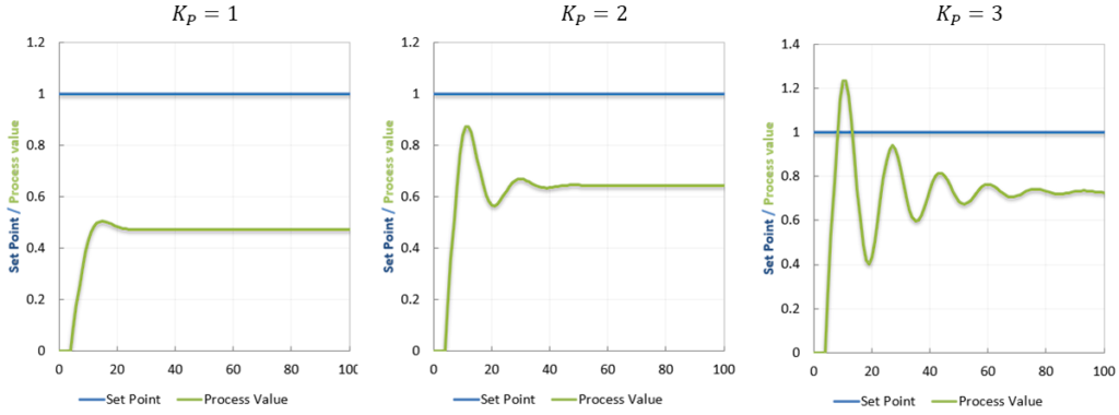
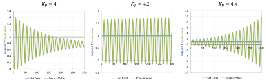
2. Increase $K_P$ until you reach undamped response, which for my particular system happens to be $K_P = 4.2$ .

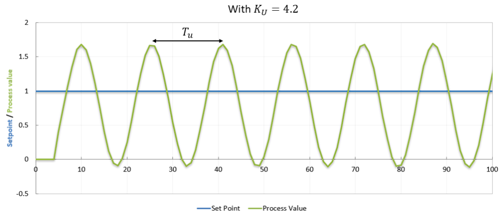
3. Record the Ultimate Gain ( $K_U = 4.2$ ), which is the proportional gain at the moment of undamped response and its corresponding Ultimate Period of oscillation ( $T_U = 15 s$ ) in seconds.

4. Utilize the parameters directly extracted from the Ziegler-Nichols table using the two values previously obtained. Referencing the table below, you can explore various control configurations, ranging from a simple P control to combinations of P, I, and D. It’s worth noting the table’s organization, featuring columns for both $T_I$ and $T_D$ , along with separate columns for the corresponding $K_I$ and $K_D$ values, depending on the parameter needed.

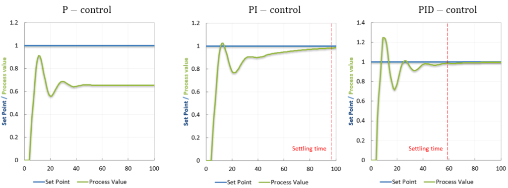
You can integrate the obtained $K_P$ , $T_I$ , and $T_D$ (or $K_I$ and $K_D$ ) into your system. Presented below are the outcomes for my particular system employing either P, PI, or PID control. While tuning all three parameters might offer optimal performance, it’s prudent to exercise caution when tuning the derivative term in the PID controller. Various factors, such as noise interference and unprecise sampling timing in discrete measurements, can introduce instability. Despite this, the inclusion of the derivative term theoretically yields the best results, as demonstrated by the settling times showcased below.

3. Ziegler-Nichols open-loop tuning method

The Ziegler-Nichols open-loop tuning method is quite a popular technique for PID controllers. The basic test requires that the response of the system be recorded as a function over time, preferably in some sort of plot as shown here. From there, you can determine the valeus of these parameters and calculate the tuning constants, by using the following procedure:

Create an open-loop test.
From the process response curve, determine the time delay ( $L$ ), or also called dead time or lag.
Measure the time constant $T$ . To do this accurately, take the time difference between the intersection at the end of the time delay and where it is reaching 63% of its total change.
Measure the value that the response reaches at steady-state, and note the step change itself, $X_0$ (the height of the step change).
Determine the tuning constants in the table below by using the the Ziegler-Nichols open-loop tuning equation: $K_0 = \frac{X_0}{K}\frac{\tau}{L}$

Advantages:

Quick and easy.
Popular method.
Less disruptive than the Ziegler-Nichols closed-loop tuning method.

Disadvantages:

The values $T_I$ and $T_D$ are based solely on the proportional measurement.
It does not work for $I$ , $D$ and $PD$ controllers.
Approximations of the gains may not work for different systems.

4. Cohen-Coon tuning method

The Cohen-Coon tuning method corrects the slow, steady-state response given by the Ziegler-Nichols method when there is a large dead time $L$ , relative to the time constant $\tau$ . This method only works in practice if L is large, otherwise unreasonably large controller gains will be predicted. Hence it only works for first-order models with a time delay.

It has a similar procedure as the Ziegler-Nichols open-loop tuning method, but note that the step change can only be introduced when the system is at steady-state.

For the Cohen-Coon method, there is again a set of predetermined settings to get a minimum offset and a standard decau ratio of 1/4 WDR. This eans that the amplitude of oscillations reduces by 75% with each cycle. This creates a faster response, but can also be more oscillatory. With the values of $K, L$ and $T$ , you can find the right parameters to optimize Cohen-Coon predictions in this table.