Updated 14 October 2024

Published 14 October 2024

Antiferromagnetic Spin Configuration – Hematite

1. Introduction

Magnetic materials are classified based on the presence or absence of ordered magnetic moments in the absence of an external magnetic field. The classifications include diamagnetic, paramagnetic, ferromagnetic, ferrimagnetic, and antiferromagnetic materials. Among these, ferromagnetic and ferrimagnetic materials exhibit finite spontaneous magnetization and are attracted to an external magnetic field. Diamagnetic materials have a total magnetization of zero; however, they possess a negative magnetic susceptibility, meaning they are repelled by an applied magnetic field by orienting their magnetic moments opposite to the direction of the external field. In paramagnetic and antiferromagnetic materials, the total magnetization is also zero, but this is due to the random or antiparallel orientation of their magnetic moments. All the classifications are illustrated in Figure 1.

The magnetic susceptibility (or magnetization) depends on temperature, as shown in Figure 2. With increasing temperature, the orientation of magnetic moments becomes more randomized, and this behavior is best described by the Curie-Weiss law. Below the Curie temperature ( $T_C$ ) and the Néel temperature ( $T_N$ ), the ferromagnetic susceptibility diverges, while the susceptibility of antiferromagnetic materials is strongly influenced by the orientation of the applied magnetic field relative to the orientation of the material’s magnetic moments.

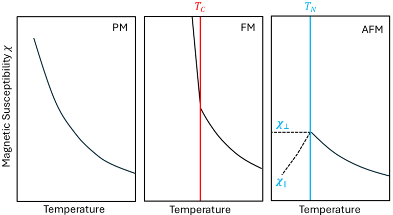
When an external magnetic field is applied parallel to the axis of the antiparallel spins (the easy axis of the antiferromagnet), the field competes primarily with the strong exchange interaction that maintains the antiparallel alignment of the spins. In this case, the spins aligned with the field will follow it, while the antiparallel spins will resist reorientation. Consequently, the magnetic susceptibility remains relatively low because the moments are locked in place. At low temperatures, thermal fluctuations are negligible, and the exchange interaction dominates. However, at higher temperatures, thermal energy begins to compete with the exchange interaction holding the spins in their antiparallel alignment. As a result, the magnetic susceptibility increases, as the spins can more easily cant due to weakened antiferromagnetic coupling, allowing for greater spin canting in response to the field.

When the magnetic field is aligned perpendicular to the antiferromagnetic axis, it causes more significant canting of the magnetic moments, making them more easily rotated away from the easy axis. In this orientation, the magnetic susceptibility is higher, and the effect of temperature is negligible (below $T_N$ ).

1.1 Superexchange interaction

I have mentioned “exchange interaction” several times; it is an effective interaction that arises from the interplay between the Pauli exclusion principle and Coulomb repulsion. This interaction leads to a preference for certain spin alignments, either parallel or antiparallel. I have written a detailed post on this topic, titled “Exchange Interaction.” The exchange interaction is described using the Heisenberg model, which expresses the energy of a system of spins in terms of their pairwise interactions. The Hamiltonian can be written as:

$H = -J\sum_{<i,j>}S_i \cdot S_j$

where $S_{i,j}$ are the spin vectors at site $i$ and $j$ . $J$ is the exchange constant that determines the nature of the interaction:

If $J>0$ , the interaction is ferromagnetic (favoring parallel spins).
If $J<0$ , the interaction is antiferromagnetic (favouring antiparallel spins).

In many antiferromagnetic materials, superexchange interaction is a common mechanism. This occurs when the spins of electrons on adjacent atoms interact indirectly through an intermediate nonmagnetic atom, such as oxygen. For example, in transition metal oxides like manganese oxide (MnO), the magnetic ions (Mn²⁺) do not interact directly with each other. Instead, their interaction is mediated by the oxygen ions, leading to an antiparallel alignment of their spins. Figure 3 illustrates the superexchange interaction. Other mechanisms, such as the RKKY interaction (Ruderman-Kittel-Kasuya-Yosida interaction) and Kondo interaction, also exist but are not covered here.

2. Hematite crystal structure

The most well-understood type of antiferromagnet is the uniaxial antiferromagnet, which features a well-defined easy axis. In the absence of an external magnetic field, the spins align along this easy axis. Typical examples of uniaxial antiferromagnets include MnF₂, FeF₂, and α-Fe₂O₃. While the uniaxial nature describes the magnetic symmetry rather than the crystal structure, understanding the unit cell geometry of antiferromagnets is still valuable to than understand the magnetic structure of the material.

2.1 Unit Cells

A unit cell represents the smallest repeating structure that contains atoms with magnetic moments aligned in alternating opposite directions, resulting in no net macroscopic magnetization. There are various types of unit cells, such as those depicted above. Imagine placing a spin-up moment at each vertex of a cubic unit cell and a spin-down moment in the center. Repeating this unit cell throughout the material will yield an antiferromagnet with no net magnetization.

One interesting material is hematite (α-Fe₂O₃). This antiferromagnet is one of the most abundant iron ores on Earth and is widely available. It serves as the primary source of iron for steel production and can be found in large deposits in many parts of the world, including on other planets such as Mars. Due to its abundance and its extensive use in various processes, hematite’s characteristics are well known.

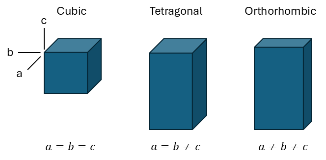
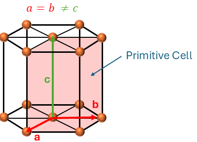
Hematite can be indexed with a hexagonal unit cell, having parameters $a = b = 5.038 Å$ and $c = 13.77 Å$ . The hexagonal unit cell is depicted in Figure 6, but it is not the smallest possible unit cell that can completely describe the crystal structure; that would be the primitive unit cell.

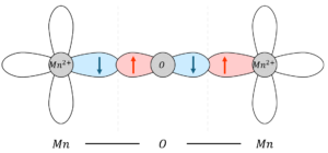
Within this primitive unit cell, layers of oxygen ions are hexagonally packed, with layers of Fe³⁺ ions in between, arranged in a six-fold ring. The magnetic moments of the Fe³⁺ ions are aligned in opposite directions across alternating lattice planes (the A and B sublattices), leading to cancellation of the spins. However, this cancellation is not maintained at room temperature. At this temperature, there is weak ferromagnetic behavior, originally attributed to defects in the crystal structure, but later proved to be not the case. To understand this phenomenon, we need to delve deeper.

2.2 Morin Transition

In 1958 and 1960, Dzyaloshinskii and Moriya demonstrated that canting of the spin sublattices occurs due to anisotropic exchange interactions (we now call this the Dzyaloshinskii-Moriya Interaction or DMI for short)[3][4], which slightly tilt the spin sublattices. This results in a small but measurable spontaneous magnetization.

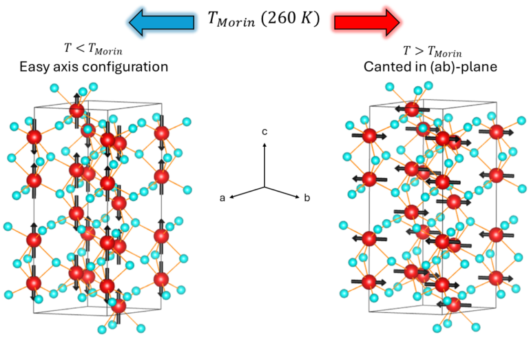
As the temperature decreases (below approximately 260 K), the magnetization nearly vanishes (and would likely approach zero in a perfect crystal). This transition, named after Morin, was observed as a decrease in magnetic susceptibility below 250 K. Powder neutron diffraction studies revealed that this effect is caused by a change in the alignment of spin moments. Below the Morin transition temperature ( $T_M$ ), the spins are aligned parallel to the crystallographic c-axis. When the temperature rises above $T_M$ , the spins reorient to lie along the basal plane (perpendicular to the c-axis) as illustrated in Figure 7 that show the primitive unit cell of hematite, with iron in red, and oxygen in blue.

This leads to two distinct types of antiferromagnets: the easy axis antiferromagnet (below $T_M$ ) and the easy-plane antiferromagnet (above $T_M$ ), each exhibiting unique magnetic properties.

Another noteworthy characteristic of hematite is its high Néel temperature $T_N\approx 950 K$ , which indicates that it can withstand significant heat before losing its magnetic properties and transitioning into a paramagnet.

3. Antiferromagnetic Resonance

In this section, we explore the dynamics of antiferromagnets under external excitation, focusing on antiferromagnetic resonance (AFMR). AFMR occurs when the magnetic sublattices in an antiferromagnet undergo precession in response to an external oscillating magnetic field. This phenomenon is similar to ferromagnetic resonance (FMR), but the setup differs significantly. To summarize the key differences:

A typical FMR setup uses a Vector Network Analyzer (VNA) to generate various frequencies ( $h_{rf}$ up to 50 GHz) and a magnet to create a static field ( $H$ ) up to 1 or 2 tesla.
For AFMR, a high-frequency microwave source ( $h_{rf}$ ) is needed to excite the magnetic sublattices in antiferromagnets. Due to the strong exchange interaction in antiferromagnets, the required frequency is typically in the range of 100 GHz to several THz. Additionally, a strong static magnetic field ( $H$ ), often exceeding 10–16 tesla, is necessary to lift the degeneracy of the resonance modes and distinguish between the high- and low-frequency components.

To achieve these experimental conditions, a specialized setup is required to measure AFMR signals. In my previous post, I discussed the experimental setup I used, which is an Electron Paramagnetic Resonance (EPR) system that was modified to measure the inverse spin Hall effect (V_ISHE) at the sample surface. While this setup can reach high fields and frequencies, it has limitations, which I outlined in that post.

Before we begin with AFMR, it’s essential to first understand the magnetic configuration of the materials at equilibrium, in the absence of an external field. Once we establish this, we can examine how applying a static magnetic field alters the behavior of hematite in its two distinct configurations, namely below and above the Morin transition.

3.1 Magnetic configuration at equilibrium

Alongside hematite, which displays different configurations based on temperature, we also added a third example, namely Yttrium Orthoferrite (YFeO₃), an antiferromagnet that exhibits unique resonance behavior due to its orthorhombic crystal structure and magnetic anisotropy. Together, these examples will allow us to explore a wider range of antiferromagnetic behaviors.

The magnetic configurations of these antiferromagnets at equilibrium are illustrated in Figure 8. The figure consists of three columns, each representing one of the antiferromagnets: hematite below the Morin transition, hematite above the transition, and YFeO₃. The crystallographic axes are labeled as a, b, and c. Note that the axes for YFeO₃ are rotated 90 degrees clockwise relative to those of hematite for ease of comparison (because the growth direction of the crystals is along the vertical axis upwards).

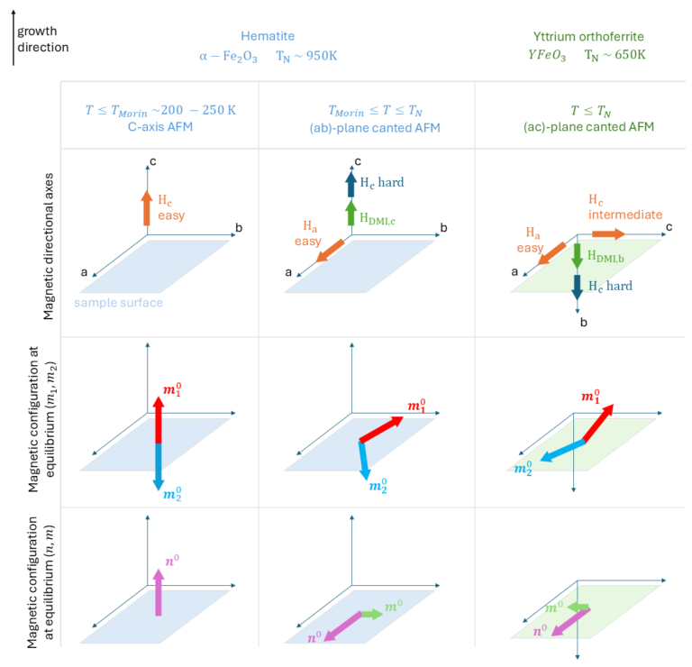
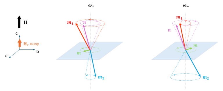
In the first row of Figure 8, the magnetic axes of each antiferromagnet are depicted. The easy-axis anisotropy is shown in orange, the hard axis in dark blue, and the Dzyaloshinskii-Moriya interaction (DMI) axis in green. The surface planes are indicated as well: for hematite, it lies in the (ab)-plane, while for Yttrium Orthoferrite, it is in the (ac)-plane.

The second row represents the two magnetic sublattices, denoted by their respective magnetizations $\textbf{M}_1$ (red) and $\textbf{M}_2$ (blue). In the easy-axis configuration, the magnetizations align antiparallel along the c-axis, with $\textbf{M}_1$ typically pointing upward. For hematite above the Morin transition, the spins reorient to the a-axis, and the DMI causes a slight canting towards the b-axis, keeping the sublattices within the surface plane. In YFeO₃, both sublattices align along the easy-(a)-axis with a small canting along the intermediate-(c)-axis, while still lying in the (ac)-plane.

In the third row, we illustrate the same configuration as the second, but with the Néel vector $\textbf{n}$ (pink) and the net magnetization $\textbf{m}$ (light green) at equilibrium. These quantities are derived from the two sublattice magnetizations, $\textbf{M}_1$ and $\textbf{M}_2$ , using the following equations:

$\textbf{n}=\frac{\textbf{M}_1-\textbf{M}_2}{2}$

where $M_{i}$ is magnetization of sublattice $i$ .

The second term is the magnetization vector, $\textbf{m}$ , which is the net magnetization of the system, defined as:

$\textbf{m}=\frac{\textbf{M}_1+\textbf{M}_2}{2}$

In an ideal antiferromagnet, the sublattice magnetizations cancel each other out, resulting in $\textbf{m} = 0$ . However, due to spin canting or interactions like the Dzyaloshinskii-Moriya interaction (DMI), a small net magnetization $m\textbf{m}$ can emerge, leading to weak ferromagnetism in some cases.

3.2 Easy-axis hematite

3.2.1 External field parallel to the easy-axis

When lowering the temperature below the Morin transition, the spins align along the easy c-axis, which I measured to be around $H_c=0.017 T$ , a value much smaller than the exchange field $H_E=1000 T$ . (Note that I should use Tesla for $\mu_0H$ ). Kittel and Keffer [5] studied collinear antiferromagnets with uniaxial easy-axis magnetic anisotropy in the previous century, deriving the following expression for the resonance frequency:

$\omega_{\pm}=\pm\gamma\mu_0H\pm\gamma\mu_0\sqrt{H_c(H_c+2H_E)}$

Where $\omega$ is the angular frequency, and $\gamma \approx 1.76*10^{11}$ is the gyromagnetic ratio, and $\mu_0H_E = 1000 T$ and $\mu_0H_c = 0.017 T$ are the exchange field and anisotropy field along the c-axis, respectively. From this equation, two unique features of antiferromagnets can already be observed:

without a static external magnetic field ( $H$ ), they exhibit a finite resonance frequency different from zero. This behaviour arises from the internal exchange field and the anisotropy field, inherent to antiferromagnets. In the case of hematite, I calculated the frequency to be around $\omega/2\pi =163$ GHz.
The second interesting observation is that we have two field-dependent modes, namely the higher-frequency mode $\omega_+$ (HFM), and the lower-frequency mode $\omega_-$ (LFM). In the absence of an external field, both modes are degenerate, meaning they share the same frequency and energy. This degeneracy is broken when the external field is increased (along the easy axis), causing the two sublattices to respond differently, as is shown in Figure 9. As a result, $\omega_+$ increases, while $\omega_-$ decreases with an increasing external magnetic field. The ratio of the radii of precession of the sublattices $\textbf{M}_1$ over $\textbf{M}_2$ is unequal for the two modes, and it depends on the material’s exchange field and anisotropy field.

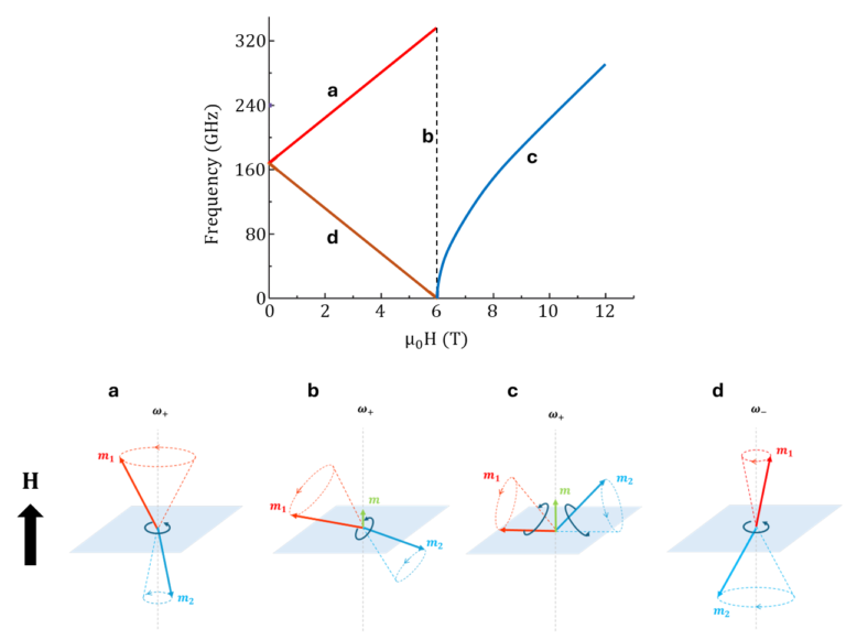
Figure 9 shows that the HFM (a) is increased $\gamma\mu_0H$ and the LFM (d) is reduced by $\gamma\mu_0H$ . This can be explained in an intuitive way, by looking at Figure 10. In the higher frequency mode, the top magnetization $\textbf{M}_1$ , parallel to $\textbf{H}$ , is driving the motion while $\textbf{M}_2$ is rather just following the exchange field of $\textbf{M}_1$ . From the point of $\textbf{M}_1$ , the effective field, composed of exchange and anisotropy fields, is parallel $\textbf{H}$ . Hence, an increase of $\textbf{H}$ results in a higher effective field, thus increasing the resonance frequency of $\textbf{M}_1$ , and the frequency of the whole system.

In the lower frequency mode, $\textbf{M}_2$ is leading the motion. However, the effective field of $\textbf{M}_2$ are antiparallel to $\textbf{H}$ . Thus, an increase of the external field will lead to a decrease of the effective field of $\textbf{M}_2$ , and the resonance frequency of the lower frequency mode.

Be aware that this only counts until the spin flop field $H_{cr}$ (for α-Fe₂O₃: $H_{cr} \approx 5.95$ T).

Spin Flip: Critical field resonance

After the spin flop field, $H_{cr}$ , the two magnetization vectors are degenerate again, with respect to the external field. This should result in a single resonance line. The magnetization configuration at the spin flop is illustrated in Figure 9 (b) and (c). In the spin flop region, it has the same precessional motion as a ferromagnet, hence it is also called the quasi-ferromagnetic regime (QFM). Nagamiya et al. [6], solved the LL-equation for the magnetization in the spin flop configuration, and found that the AFMR condition above this critical field is described as:

$\omega_{sf}=\gamma\mu_0\sqrt{(H^2-2H_EH_c)}$

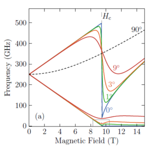
In their experiment, their theory describes the data quite well, except for the spin flop region. Here the data deviate slightly from the theoretical curves. This was later found out to be due to the misalignment of the external field, $\textbf{H}$ , with respect to the easy axis $\textbf{H}_c$ . Where a small misalignment of a few degrees can already have large consequences for the resonances in the spin flop region, as modelled in Figure 11.

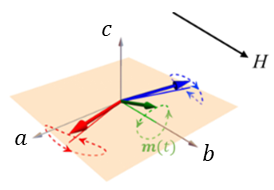
3.2.2 External field perpendicular to the easy axis

In the case we apply the field perpendicular to the easy-axis, we observe a completely different configuration, which is expressed by the equation [8]:

$\omega_{res}=\gamma\mu_0\sqrt{H^2+2H_EH_c}$

It is obvious that at zero field, it has the same finite resonance frequency of $\gamma\mu_0\sqrt{2H_EH_c}$ , where the magnetization of the sublattices lie in the easy-(c)-axis. Applying an external field will tilt the magnetizations out of their easy-axis configuration, as shown in Figure 12.

3.3 Easy-Plane Hematite

When increasing the temperature above the Morin transition, due to the introduction of the DMI field, the spins reorient themselves along the basal (ab)-plane, perpendicular to the c-axis. This type of antiferromagnet is also called the easy-plane AFM, where instead of a single axis, it can ideally point in any direction in the (ab)-plane. However, in hematite, there is a (very) small easy axis anisotropy along the a-axis, which I measured to be roughly $H_a = 7.3\times 10^{-5} T$ .

As shown in Figure 13, the presence of DMI will cant the sublattice magnetizations $\textbf{M}_1$ and $\textbf{M}_2$ toward the b-axis at equilibrium, and precess elliptically around the canted directions, resulting in an elliptical circulating $\textbf{m}(t)$ around the b-axis. Because the elliptical trajectory of $\textbf{m}$ has a finite projection along the a-axis direction, microwave magnetic field polarized along the Néel vector, can effectively drive this resonance mode. Thus, when applying the external static magnetic field along the a-axis, we obtain two eigenmodes, that are non-degenerate, meaning they do not have the same frequency and energy at equilibrium, thus giving a lower-frequency mode $\omega_-$ and high-frequency mode $\omega_+$ [10]:

$\omega_- = \gamma\mu_0\sqrt{2H_EH_a+H(H+H_{DMI})}$

$\omega_+=\gamma\mu_0\sqrt{2H_E(H_c+H_a)+H_{DMI}(H_{DMI}+H)}$

where $\gamma$ is the gyromagnetic ratio, $H_E$ is the exchange field, $H_a, H_c$ is the anisotropy field along the easy-a-axis and hard-c-axis, respectively, and $H_{DMI}$ is the DMI field.

Figure 14(a) and (b) show the model and actual data points. We observe that the low-frequency mode ( $H//a$ ), in the absence of an applied field, depends only on the exchange field and anisotropy field, and not on the DMI field. Since the anisotropy is very small, the resonance frequency decreases to approximately 11 GHz, making it accessible to most commercial microwave units.

4. Summary

Hematite is an intriguing material with an hexagonal unit cell and a Morin transition around 260 K, where its spins reorient from the c-axis to the basal plane. However, the main focus of this article is on antiferromagnetic resonance (AFMR), where the sublattices precess under high-frequency fields. Below the Morin transition, hematite exhibits distinct resonance modes—higher and lower frequency—both influenced by external magnetic fields. Above the Morin transition, these modes become non-degenerate in zero field due to the Dzyaloshinskii-Moriya interaction (DMI) and the hard axis. Notably, the lower frequency mode reaches 11 GHz, making it accessible to typical FMR setups.

From what we have seen, the spin dynamics in antiferromagnets has much shorter timescale than that of ferromagnets. This offers attractive properties for potential applications in ultrafast devices. The frequency of typical antiferromagnetic dynamics falls in the THz region, which is critical for developing the AFM-based oscillator in spin-based nanoscale devices.

As this post grew longer and less coherent, I’ll continue discussing advanced techniques like spin pumping, the inverse spin Hall effect, and Yttrium Orthoferrite in my next article, expanding on antiferromagnetic resonance.

4.1 References

[2] Z. Jian et al., The magnetic and Color Reflectance Properties of Hematite: From Earth to Mars, Reviews of Geophysics, vol 60, 1, (2022).

[3] T. Moriya, Phys. Rev., vol. 117, 635, (1960).

[4] I. E. Dzyaloshinskii, Zh. Eksperi,. i Teor. Fiz., vol. 33, 1454, (1957).

[5] F. Keffer and C. Kittel, Theory of Antiferromagnetic Resonance, Phys. Rev., vol. 82, 565, (1951).

[6] T. Nagamiya and T. Nishikubo, Dynamics of the spin flop in antiferromagnet, Phys. Rev. Lett., vol. 31, 1061, (1973).

[7] M. Ross, Spin Dynamics in an Antiferromagnet, PhD Thesis, TU Munchen, (2013).

[8] . M. Hagiwara, K. Katsumata, H. Yamaguchi, M. Tokunaga, I. Yamada, M. Gross, P. Goy, A Complete Frequency-Field Chart for the Antiferromagnetic Resonance in MnF2. International journal of infrared and millimeter waves, vol. 20, (4) p. 617-622, (1999).

[9] Hailong Wang, Yuxuan Xiao, Mingda Guo, Eric Lee-Wong, Gerald Q. Yan, Ran Cheng, and Chunhui Rita Du, Spin Pumping of an Easy-Plane Antiferromagnet Enhanced by Dzyaloshinskii–Moriya Interaction, Phys. rev. Lett., vol. 127, 117202, (2021).

[10] R. Lebrun et al., Long-distance spin-transport across the Morin phase transition up to room temperature in ultra-low damping single crystals of the antiferromagnet α-Fe2O3, Nat. comm., vol. 11, 6332, (2020).

Post Views: 10

0 0 votes

Article Rating

0 Comments

Oldest

Newest Most Voted

Inline Feedbacks

View all comments