Updated 24 May 2024

Published 20 April 2024

Micromagnetics – An Introductory Overview

1. Micromagnetics

Micromagnetics is a field in physics that deals with the behaviour of magnetics at a sub-micrometer dimension. This theory is based on the assumption that the length of the magnetization vector is constant, and that the energy varies slowly at the atomic scale. This will break down when approaching the atomic size, but it is suitable for resolving magnetic structures, such as domain walls, vortices and more. Due to this assumption of constant magnetization length, it does not work for temperatures far from the Curie temperature. Its principles were first outlined in 1949 by William Fuller Brown.

It all resolves around minimizing he energy by, for example, solving the dynamic equation of motion. The dynamics of the magnetization vector in an external field are governed by the Landau-Lifshitz-Gilbert equation [1]:

$\frac{d\textbf{m}}{dt} = -\gamma_0(\textbf{m}\times\textbf{H}_\textrm{eff}) + \alpha\textbf{m}\times\frac{d\textbf{m}}{dt}\ ,$

where $\textbf{m} = \frac{\textbf{M}}{M_s}$ is the normalized magnetization vector, $\gamma_0$ is the gyromagnetic ratio, $\alpha$ is the Gilbert damping parameter, and $\textbf{H}_\textrm{eff}$ is the effective field. The latter one consists of external magnetic field, and other contributions that will be described in later sections down here. $\textbf{H}_\textrm{eff}$ can be represented as the first derivation of the total energy density with respect to the magnetization.

$\textbf{H}_\textrm{eff} = -\frac{1}{\mu_0 M_s}\frac{\partial\textbf{E}}{\partial\textbf{m}} \,$

where $M_s$ is the saturation magnetization, and $\textbf{E}$ is the total energy of the ferromagnetic element, which includes exchange, magnetic anisotropy, magnetostatic, and Zeeman energy contributions.

Most often, for numerical calculations, the Gilbert equation [2] is converted into the following form:

$\frac{d\textbf{m}}{dt} = \frac{1}{1+\alpha^2}\left[-\textbf{m}\times\gamma_0\textbf{H}_\textrm{eff}- \alpha (\textbf{m}\times\textbf{m}\times\gamma_0\textbf{H}_\textrm{eff}) \right]$

2. Magnetic interactions

The total energy of a ferromagnet with respect to the magnetization depends on many physical effects. Some of them have classical descriptions, such as the Zeeman energy. Other effects have a quantum mechanical origin, and should therefore be converted to the continuous limit of micromagnetism, such as the exchange energy and the anisotropy energy. In this article I will not derive the micromagnetic expressions from the Hamiltonians for all the terms, but will only show the effective magnetic field terms. For full derivations, I will refer you to the PhD dissertation of [3] or on the website of micromagnetics.

2.1 Total effective magnetic field

The dynamics of the system are defined by the effective magnetic fields on each point of the ferromagnet. In the previous section a description on the equations was given, in this equation an effective magnetic field is required that consists of a summation of each one of the fields corresponding with a magnetic interaction,

$\textbf{H}_\textrm{eff} = \textbf{H}_\textrm{exc} + \textbf{H}_\textrm{ani} + \textbf{H}_{\textrm{DMI}{\bot}} + \textbf{H}_\textrm{zee}\ ,$

where $\textbf{H}_\textrm{exc}$ is the exchange interaction effective field, $\textbf{H}_\textrm{ani}$ is the anisotropy effective field, $\textbf{H}_{\textrm{DMI}{\bot}}$ is the perpendicular DMI effective field, $\textbf{H}_\textrm{zee}$ is the Zeeman term.

These terms were proposed in [4][5], where they derived it by using semi classical approximations. Each of these interactions has an energy associated with it. Through damping, the micromagnetic approach will try to minimize the total energy of these terms. Each of these interactions will be briefly described in the following sections, except the torque. This term should also be added as well into the effective magnetic field, but it will be described in it’s own section.

2.2 Exchange interaction

Ferromagnetism is caused by the exchange interaction between the electrons. The elementary magnetic moments in ferromagnets are subjected to an exchange interaction. This is a quantum mechanical effect that aligns neighboring spins for a positive exchange constant and it creates a uniform magnetization on a macroscopic scale as illustrated in Figure 2. A negative constant would lead to an anti-ferromagnetic state as shown in . In the continuous limit, the exchange interaction is described as an effective magnetic field term with the following equation}:
$\textbf{H}_{\textrm{exc}} = \frac{2}{\mu_0}\frac{J}{M_s}\nabla^2 \textbf{m}\ ,$
with $\mu_0$ denotes the permeability of free space, $M_s$ the saturation magnetization, the corresponding exchange interaction constant $J$ and $\textbf{m}$ the normalized magnetic moment.

2.3 Anisotropy

A crystal lattice favours or impedes the magnetization in a certain preferential direction. This effect is called anisotropy and it has its origin in the material spin-orbit interactions [7]. The magnetization will prefer to align itself along the easy axis to minimize the energy. The anisotropy is described in the following term of the effective magnetic field.
$\textbf{H}_{\textrm{ani}} = \frac{2}{\mu_0}\frac{K}{M_s}\textbf{m}z\ ,$
where K is the anisotropy constant and the rest of the parameters are the same as above.
Material anisotropy is responsible for permanent magnetization. Soft and hard magnets are characterized by small and large magnetic anisotropy respectively.

2.4 Dzyaloshinskii-Moriya interaction

Dzyaloshinskii-Moriya interaction is an anti-symmetric exchange, as shown in Figure 3, that originates from a combination of large spin-orbit coupling (SOC) and broken inversion symmetry. This chiral interaction is a key aspect of the creation of skyrmions. I. Dzyaloshinskii and T. Moriya [8][9] showed that the DMI between two spins can be expressed with the Hamiltonian:
$\mathcal{H}_{\textrm{DM}}=-\textbf{D}_{12}\cdot(\textbf{S}_1\times\textbf{S}_2)\ ,$
where $\textbf{S}_1$ and $\textbf{S}_2$ represent the two spin atoms and $\textbf{D}_{12}$ is the DMI vector. There are two types of DMI, one that can exist in the bulk of certain materials, and the second type is at the interface between a ferromagnet with a heavy metal layer. Both types will be explained below.

2.4.1 Bulk DMI

In a bulk material, the DMI vector is shown in as $\textbf{D}_{12} = \textbf{D}_\textrm{bulk} = D_\parallel\textbf{r}_{12}$ , where $D_\parallel$ is the strength of the bulk DMI and $\textbf{r}_{12}$ is the vector between both spin atoms [10]. The bulk DMI originates from the breaking of the inversion symmetry in the non-centrosymmetric lattice of a bulk material itself [11]. It can be seen from Figure 4(a), that this is also called the parallel ( $\parallel$ ) DMI, as it is parallel to the vector between $\textbf{S}_1$ and $\textbf{S}_2$ .
The corresponding effective magnetic field term is derived to be [13]:
$\textbf{H}_{\textrm{DMI}\parallel} = -\frac{2}{\mu_0}\frac{D_{\parallel}}{M_s}(\nabla\times\textbf{m})\ ,$
where the parameters are the same as described above.

2.4.2 Interfacial DMI

In an interface, the mechanics are somewhat different. The interfacial DMI vector is shown in as $\textbf{D}_{12} = \textbf{D}_\textrm{int} = D_\bot(\textbf{z}\times\textbf{r}_{12})$ , where $D_\bot$ is the strength of the interface DMI, $\textbf{r}_{12}$ is the vector between both spin atoms and $\textbf{z}$ is the interface normal direction [10]. In this case, the inversion symmetry is broken at the interface between the ferromagnetic film with a heavy metal layer with a strong SOC [12]. This type of DMI, is also called the perpendicular ( $\bot$ ) DMI, as the vector is along ( $z\times r$ ).
The corresponding effective magnetic field term is derived to be [13]:
$\textbf{H}_{\textrm{DMI}\bot} = -\frac{2}{\mu_0}\frac{D_{\bot}}{M_s}((\nabla\cdot\textbf{m})z - \nabla \textbf{m}_z)\ ,$

where the parameters are the same as described above.

2.5 External field

In the field of magnetism, in addition to the magnetic induction (\textbf{B}), there is another quantity called the magnetic field (\textbf{H}), that differ on the material response, that produces its own magnetization (\textbf{M}). This gives the following equation:
$\textbf{B} =\mu_0(\textbf{H} + \textbf{M})\ ,$
where $\mu_0$ is the permeability of free space and the rest is the same as described above. By substituting \textbf{B} into the LLG equation, the following partial cross product is obtained
$\textbf{M}\times\textbf{B} = \mu_0\textbf{M}\times\textbf{H} + \mu_0\textbf{M}\times\textbf{M} = \mu_0\textbf{M}\times\textbf{H}\ .$
Because ( $\textbf{M}\times\textbf{M}) = 0$ , there is no need to account for the material response $\textbf{M}$ . Hence, \textbf{B} is only proportional to $\textbf{H}$ with a constant $\mu_0$ . This is called the Zeeman term of the magnetic field ( $\textbf{H}_\textrm{zee}$ ).

2.6 Spin-transfer torque

2.6.1 Spin-polarized current

In a ferromagnet, the spin occupation is imbalanced as shown in Figure 5. For a given energy level, there is more of one spin compared to the other. In this example, the d-band with spin $\uparrow$ is nearly completely filled, while the band with spin $\downarrow$ is nearly empty. Any itinerant electrons with a spin $\downarrow$ will get trapped by the empty states, while the electrons with a spin $\uparrow$ are free to move. This creates a current that has a majority of a certain spin, also known as a spin-polarized current. The polarization is not perfect as there are still free states available in the d-band, but the effect is significantly in favour of the spin $\uparrow$ polarized current.

2.6.2 Spin-transfer torque

In a ferromagnet, the spins of electrons are bound to the atoms of the lattice, whereas in a metal, the spin current of the electrons flows across the material. Spin transfer torque refers to the interaction between the spins of the ferromagnet and those of the metal. Due to the conservation of momentum, this interaction results in torques of equal magnitude but opposite signs acting on these spins.

Adding the torque to Eq. (??) results in the following:

(1) $\begin{equation*}\frac{d\textbf{M}}{dt} = -\frac{1}{1+\alpha^2}\textbf{M}\times\gamma_0\textbf{H}_\textrm{eff}- \frac{1}{1+\alpha^2}\frac{\alpha}{M_s}(\textbf{M}\times\textbf{M}\times\gamma_0\textbf{H}_\textrm{eff}) + \textbf{T}\ ,\end{equation*}$

where the torque ( $\textbf{T}$ ) is expressed as [15]:

(2) $\begin{multline*}\textbf{T}= \frac{1}{1+\xi^2}\left[-\frac{n_0}{M_s}\frac{\delta\textbf{M}}{\delta t} + \frac{\xi n_0}{M_s^2}\textbf{M}\times\frac{\delta\textbf{M}}{\delta t}-\frac{\mu_BP}{eM_s^3}\textbf{M}\right.\\ \left.\times[\textbf{M}\times(\textbf{j}_e\cdot\nabla)\textbf{M}] -\frac{\mu_BP\xi}{eM_s^2}\textbf{M}\times (\textbf{j}_e \cdot\nabla)\textbf{M}\right] \ ,\end{multline*}$

where $n_0$ is the local equilibrium spin density, $M_s$ is the magnetization saturation, $\mu_B$ is the Bohr magneton, $P$ is polarization of the spin-polarized current, $e$ is the electron charge, $\textbf{j}_e$ is the current density and $\textbf{M}$ is the magnetization. $\xi$ models the strength of the electronic diffusion in the metal. $\xi$ is zero if the current is transported ballistically and different from zero if electron scattering is present.

2.6.3 Conversion into effective field

According to Zhang and Li [15], the torque consists of four terms, as shown in Eq. (2). The first two are from the magnetization variation in time and the other two describe the magnetization variation in space. However, the temporal torques can be absorbed by the redefinition of the gyromagnetic ratio and damping constant and can therefore be ignored. Hence, only the spatial magnetization part of the torque will be used. This term consists of the current density, $\textbf{j}_e$ , which is further changed to model the proposed device as will be clear in the next section. The final expression for the spatial torque is the following:

(3) $\begin{equation*}\textbf{T}=\frac{b_j}{M_s^2}\textbf{M}\times\textbf{M}\times(\textbf{j}_e\cdot\nabla)\textbf{M} + \frac{c_j}{M_s}\textbf{M}\times(\textbf{j}_e\cdot\nabla)\textbf{M}\ ,\end{equation*}$

where

(4) $\begin{equation*}b_j = -\frac{\mu_B P}{eM_s(1+\xi^2)}\ ,\ c_j = \xi b_j .\end{equation*}$

Eq. (1) can not easily be solved by the numerical integration programs. Instead, the torque can be rewritten as an effective magnetic field through several steps. To do that, the LL equation can be converted back into an LLG expression, following the steps in this post on the LLG equation, but in the reverse order. Then the torque can be rewritten as an effective field and added to the rest. Finally this LLG equation can be transformed back into the LL form to numerically solve it.

(5) $\begin{multline*}\frac{d\textbf{M}}{dt} = -\gamma_0(\textbf{M}\times\textbf{H}_\textrm{eff}) + \frac{\alpha}{M_s}\textbf{M}\times\frac{d\textbf{M}}{dt} + \\ \textbf{M}\times\left[\textbf{M}\times\frac{b_j}{M_s^2}(\textbf{j}_e\cdot\nabla)\textbf{M}+ \frac{c_j}{M_s}(\textbf{j}_e\cdot\nabla)\textbf{M}\right]\end{multline*}$

Next, Eq. (5) is made dimensionless in order to solve it numerically. Through several mathematical steps that are explained in more detail in Appendix ??, and with the aid of relationship $\textbf{M} = M_s\textbf{m}$ the following result is obtained:

(6) $\begin{multline*}\frac{d\textbf{m}}{dt} = -\gamma_0(\textbf{m}\times\textbf{H}_\textrm{eff}) + \alpha\textbf{m}\times\frac{d\textbf{m}}{dt} +\\ \textbf{m}\times \left[\textbf{m}\times b_j(\textbf{j}_e\cdot\nabla)\textbf{m} + c_j (\textbf{j}_e \cdot\nabla)\textbf{m}\right]\ ,\end{multline*}$

where $\textbf{m}$ is the dimensionless magnetization and the other parameters are the same as above. This adimensionalization avoids the usual loss of precision associated with numerical calculations, because it avoids to use large and/or small numbers.
By taking certain parameters together and rewriting the equation further, it gives the following intermediate result:

(7) $\begin{equation*}\frac{d\textbf{m}}{dt} = -\gamma_0\textbf{m}\times\left[\textbf{H}_\textrm{eff} + \textbf{m}\times\frac{\textbf{B}}{-\gamma_0} + \frac{\textbf{C}}{-\gamma_0}\right] +\alpha\textbf{m}\times\frac{d\textbf{m}}{dt}\ ,\end{equation*}$

where

(8) $\begin{equation*}\textbf{B} = b_j(\textbf{j}_e\cdot\nabla)\textbf{m} \textrm{ and }\textbf{C} = c_j(\textbf{j}_e\cdot\nabla)\textbf{m}\ .\end{equation*}$

From Eq. (7), the part inside the brackets with $\textbf{B}$ and $\textbf{C}$ can be taken into a single term $\textbf{H}_\textrm{torq}$ that describes the torque as an effective magnetic field. The final equation will be a dimensionless version in the LLG form, as given by:

(9) $\begin{equation*}\frac{d\textbf{m}}{dt} = -\textbf{m}\times(\gamma_0\textbf{H}_\textrm{eff} + \textbf{H}_\textrm{torq}) +\alpha\textbf{m}\times\frac{d\textbf{m}}{dt}\ ,\end{equation*}$

where the torque appears as an effective magnetic field is described as:

(10) $\begin{equation*}\textbf{H}_\textrm{torq} = \textbf{m}\times \left(\textbf{u}\cdot\nabla)\textbf{m}\right) + (\xi\textbf{u}\cdot\nabla)\textbf{m}\ ,\end{equation*}$

where $\textbf{m} = \frac{\textbf{M}}{M_s}$ the dimensionless magnetization and $\textbf{u} = -b_j\textbf{j}_e$ .

It can be shown that the term $\textbf{H}_\textrm{torq}$ has the same units has the magnetic field, thus it can be absorbed in the effective magnetic field equation of section 2.1. To solve the remaining standard LLG expression, it can be further transformed into the LL equation that has no time dependency on the right hand side of equation by using the transformation results obtained in the article on the LLG equation.

3. Micromagnetic modelling

A lot has changed since 1949, when W. Brown developed the mathematical model for micromagnetism. Large-scale computers are the main reason why micromagnetic modelling has been developed so rapidly. The numerical equations in the previous chapters can be integrated into a software program, that can simulate the magnetization dynamics in a 2D (and in some cases 3D) interface. I will start by giving a general overview of how I tackled this problem, and then show you more professional software tools that are worth looking into.

3.1 Self-made software

As I will not publish my own software, I will give some tips on how to tackle it. First off, to create your own program, it’s good to have a basic in coding languages, such as Python, or Fortran. Secondly, almost all the information is already available in the form of numerical equations in the previous sections. The task of the software is to solve these equations with initial parameters and specified boundary conditions.

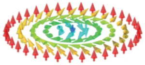
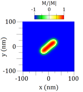
The surface can be discretized into a grid of points and the LLG equation needs to be solved at each point on this grid. For that we need to set initial conditions for each point on that grid, and specify the boundary conditions, so we do not create artifacts at the edges. The initial conditions in Figure 6 were most likely that the magnetization at all grid points, besides the center, were pointing down, indicated by the color blue (red stands for pointing up). Note that in my experiments I was simulating the interface between a ferromagnetic layer with a metallic layer, hence we have interfacial DMI, that allows skyrmions.

From here, we can calculate the effective magnetic field ( $\textbf{H}_\textrm{eff}$ ) of each point separtely, with the initial conditions given. From here the right hand side of the numerical LLG equation can be calculated. A different module performs the numerical integration of the LLG equation, using methods such as Euler, Heun and Dormand-Prince. Depending on the complexity of the system, you will find that certain methods are faster than others. Lastly, you will have to find something to display the information, this can be done through OriginLab, GNUplot, or other options available to you.

When dealing with modelling magnetic structures, you will have to create models that initialize them on your interface. The main issue is to get it to become stable. Take a skyrmion for example, which only has a small range of useable parameters, see Figure 7. When initializing the skyrmion with a number of requirements, such as the initial radius, the type (Nëel or Bloch), the magnetization direction at its center and its initial coordinates, you will have to allow it to evolve to its minimum energy configuration

3.2 Professional software tools

There are several micromagnetic simulation tools avaible, each with their own strength and capabilities. Here are some of the popular ones.

OOMMF (Object Oriented MicroMagnetic Framework): It is a widely used open-source micromagnetic simulation package developed by the National Institute of Standards and Technology (NIST). It supports various simulation techniques and models, including LLG dynamics, energy minimization, and more.

MuMax3: This is a GPU-accelerated micromagntic simulation tool developned by the DyNaMat group at the Gent University. it supports features such as parallel computing, non-uniform grids, and advanced material properties. However, you’ll need an NVIDIA graphics card for it (I got an AMD…).

MAGPAR: This is a finite element micromagnetic package that offers a range of simulation capabilities, including LLG dynamics and thermal effects. It is highly efficient and scalable.

Vampire: This shouldn’t be in the list, as it is an atomistic simulation tool for magnetic materials. However, since it is a free and open-source package i will include it in the list. It bridges the gap between micromagnetics approaches and electronic structure by treating a magnetic material at the natural atomic length scale. I’ve had the pleasure to meet the creator R. Evans and it left a great impression on me.

4. References

[1] L. Landau and E. Lifshitz, “On the theory of magnetic permeability in ferromagnetic bodies.” Phys. Z. Sowjetunio, vol. 8, pp. 153-169, 1935.

[2] T. Gilbert, “A lagrandian formulation of the gyromagnetic equation of the magnetization field.” Phys Rev, vol. 100, pp. 1243, 1955.

[3] C. Abert “Discrete Mathematical Concepts in Micromagnetic Computations” PhD. Thesis. Universitat Hamburg ,Germany, 2013.

[4] Y. Liu, D.J. Sellmyer and D. Shindo, “Handbook of advanced magnetic materials. Volume 1: nanostructural effects”, Springer, 2005.

[5] C. Abert, “Micromagnetics and spintronics: models and numerical methods.”, Eur. Phys. J. B., vol. 92, 120, 2019.

[6] NanoScience, “Noncollinear spins.”, Feb. 13, 2022. [Online] Available: http://www.nanoscience.de/HTML/research/noncollinear_spins.html [Accessed: April. 24, 2024].

[7] N. A. Spaldin, “Magnetic materials: fundamentals and applications.“, Cambridge : Cambridge University Press, 2013.

[8] I. Dzyaloshinsky, “A thermodynamic theory of weak ferromagnetism of antiferromagnetics.”, J. Phys. Chem. Solids, vol. 4, pp. 241-255, 1958.

[9] T. Moriya, “New mechanism of anysotropic superexchange interaction”, Physical review letters, vol. 4, 5, 1960.

[10] K.-W. Kim, K.-W. Moon, N. Kerber, J. Nothhelfer and K. Everschor-Sitte, “symmetric skyrmion Hall effect in systems with a hybrid Dzyaloshinskii-Moriya interaction.”, Phys. Rev. B, vol. 97, 224427, 2018.

[11] S. Muhlbauer, B. Binz, F. Jonietz, C. Pfleiderer, A. Rosch and A. Neubauer, et al., “Skyrmion Lattice in a Chiral Magnet.”, Science, vol. 14, pp. 915-919, 2009.

[12] M. Bode, M. Heide, K. von Bergmann, P. Ferriani, S. Heinze, G. Bihlmayer, A. Kubetzka, et al., “Chiral magnetic order at surfaces driven by inversion asymmetry.”, Nature, vol. 447, pp. 190-193, 2007.

[13] S. Rohart and A. Thiaville, “Skyrmion confinement in ultrathin film nanostructures in the presence of Dzyaloshinskii-Moriya interaction.”, Phys. Rev. B, vol. 88, 184422, pp. 1-8, 2013.

[14] A13ean, “Stoner model of ferromagnetism. [Online] Available: en.wikipedia.org/wiki/File:Stoner model of ferromagnetism.svg [Accessed: April 24, 2024].

[15] S. Zhang and Z. Li, “Roles of Nonequilibrium Conduction Electrons on the Magnetization Dynamics of Ferromagnets.”, Physical Review Letters, vol. 93, 12, pp. 12704, 2004.

Post Views: 47

0 0 votes

Article Rating

0 Comments

Oldest

Newest Most Voted

Inline Feedbacks

View all comments