
I own a 3D printer and regularly create items such as figurines and busts, which I then paint. For this, I use a collection of 28 colors from the Vallejo Model Color range. To store these paints, I have a rack organized into 3 rows and 16 columns.
Table of Contents
The objective of this article is to analyze the colors within my paint palette in order to identify an underlying structure that can inform a systematic and visually coherent arrangement. If achieving that means purchasing one or two additional colors, I’m happy to do so.
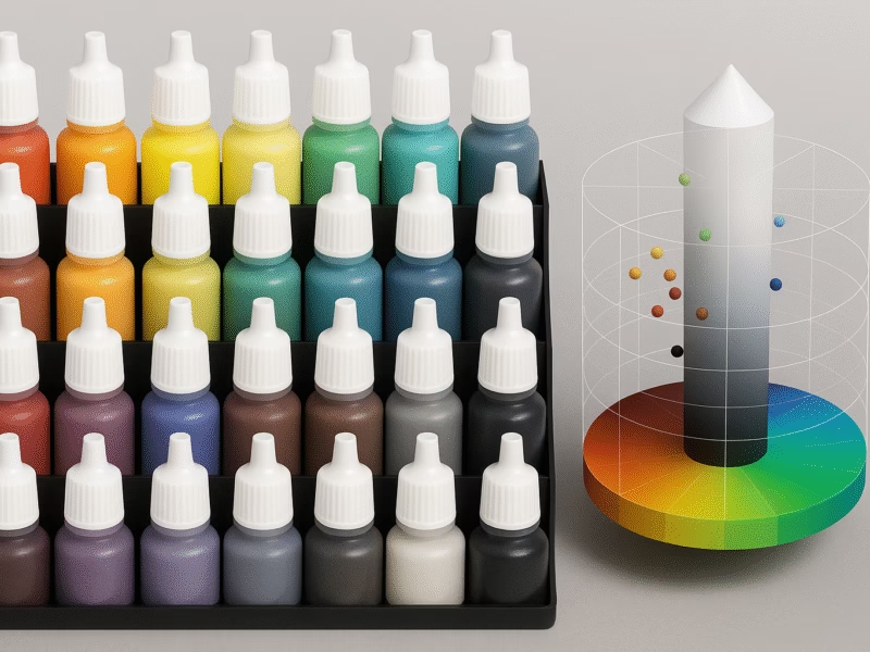
In this post, I’ll walk you through the basic idea behind the model I’m using. Starting with the Red-Green-Blue (RGB) color scheme, we can map the color of the paints into a 3D structure using the HSV (Hue, Saturation, Value) color model. Below, you’ll find an interactive 3D visualization showing where each of my paints lies within this HSV space.
Once the HSV model is introduced, I proceed to analyze the distribution of the colors using two techniques: histograms to explore value distributions, and K-Means clustering to identify natural groupings within the palette. If you are interested in what else I wrote on this topic, see my posts on K-Means Clustering for Colors and my latest post on Sorting Vallejo colors with Machine Learning.
From RGB to the HSV
Every digital color can be represented by combining Red (R), Green (G), and Blue (B) light. Each channel ranges from 0 (no intensity) to 255 (full intensity). For example, pure red is written as (255, 0, 0), white as (255, 255, 255) and black as (0, 0, 0). Instead of writing RGB values in decimal, it’s also common to use hexadecimal notation, where 255 is written as FF and 60 as 3C. Using this format, yellow—being a mix of red and green at full intensity—is represented as #FFFF00.
While RGB is widely used, a more intuitive way to describe color is through the HSV color model, which stands for Hue, Saturation, and Value. Sometimes “Brightness” is used in place of “Value”, but in this context, both refer to the same thing: the highest of the RGB components, or Cmax.
Before converting RGB to HSV, the RGB values are normalized to the range [0,1] by dividing each component by 255 (i.e., R’= R/255, and similar for G’ and B’). Based on these normalized values, we define:
\[
\begin{aligned}
C_{\text{max}} &= \max(R’, G’, B’) \\
C_{\text{min}} &= \min(R’, G’, B’) \\
\Delta &= C_{\text{max}} – C_{\text{min}}
\end{aligned}
\]
Hue
Hue describes the type of color and is computed based on which RGB component is the largest. It’s defined as:
\[
H =
\begin{cases}
0^\circ, & \Delta = 0 \\
60^\circ \times \left( \frac{G’ – B’}{\Delta} \bmod 6 \right), & C_{\text{max}} = R’ \\
60^\circ \times \left( \frac{B’ – R’}{\Delta} + 2 \right), & C_{\text{max}} = G’ \\
60^\circ \times \left( \frac{R’ – G’}{\Delta} + 4 \right), & C_{\text{max}} = B’
\end{cases}
\]
Note: If two components are tied for the maximum, the standard approach is to choose based on the order: R’ > G’ > B’.
Saturation
Saturation measures how vivid the color is:
\[
S =
\begin{cases}
0, & C_{\text{max}} = 0 \\
\frac{\Delta}{C_{\text{max}}}, & \text{otherwise}
\end{cases}
\]
Value
Value (or brightness) corresponds to the highest RGB component:
\[V=C_{max}\]
HSV model
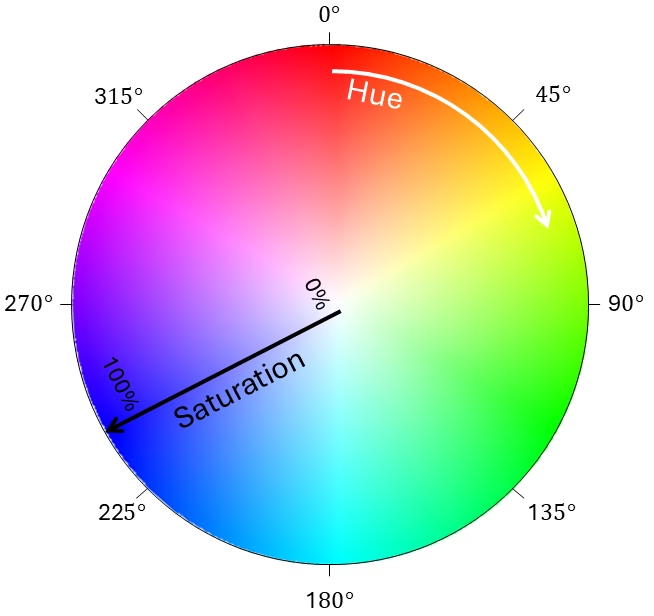
Hue in the HSV model is measured in degrees from 0° to 360°, forming a circular spectrum—red appears at both 0° and 360°. In the 2D representation of the hue-saturation plane, hue corresponds to the angle around the circle, while saturation is the radial distance from the center: fully saturated colors lie on the edge, and desaturated colors (grays) lie near the center.
To represent value, the model adds a third dimension. This creates a cylinder, where vertical position represents brightness: the bottom of the cylinder corresponds to black (value = 0), and the top represents full brightness (value = 1). Each horizontal slice of the cylinder at a given brightness level forms a 2D hue-saturation circle.
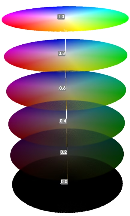
Figure 2 shows these horizontal slices taken at intervals of 0.2 in brightness. As brightness decreases, colors become darker and more muted, eventually blending into black. Thus, the full 3D HSV model is best visualized as a cylinder, where:
- Hue is the angle around the vertical axis,
- Saturation is the distance from the center axis outward,
- Value is the height along the vertical axis.
This cylindrical form helps visualize how colors shift in hue, become more or less vivid (saturation), and change in brightness—all in a single geometric structure.
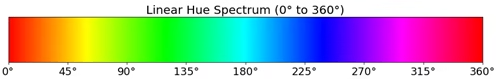
While the HSV model is naturally represented as a cylinder due to the circular nature of hue, it’s also possible to visualize the hue-saturation plane as a 2D rectangular grid, with hue on the horizontal axis (0–360° or normalized 0–1) and saturation on the vertical axis (0–1). In this projection, the circular structure of hue is lost—colors at 0° and 360° appear on opposite ends, as shown in Figure 3—but it remains a useful way to analyze and personally views better than seeing it on the inside of a colored cylinder.
Analysis of Vallejo Game Colors
My dataset consists of the 28 colors from the Vallejo Game Color set. These colors were converted into hexadecimal codes using the website encycolorpedia.com, which matches Vallejo’s color codes with their closest digital equivalents, to see which colors I have, I refer you to the interactive Figure at the top of this page. One thing I noticed is that the brightness on the digital results appears slightly lower for nearly all the colors—this could be due to my display settings, so please take the data with a grain of salt. Nevertheless, the dataset provides a solid basis for analysis.
Color distribution
Using Python’s “Colorsys” library, I converted the hexadecimal color codes into HSV and plotted the colors based on their hue and saturation. Figure 4 (left) shows this 2D distribution, where each point represents one of the 28 colors from the set. The color bar at the top illustrates the full hue spectrum at maximum saturation and brightness, providing a reference for how pure hues vary across the range.
Figure 4 (right) extends this to a 3D HSV representation. In this plot, hue and saturation remain on the horizontal axes, while the vertical axis now reflects the value (or brightness) of each color—capturing the full HSV distribution of the palette.

Clustering in Color Space
Based on the distribution of our colors, several characteristics of the palette become apparent—best visualized using histograms. A histogram, as shown in Figure 5, is a graphical representation of the frequency distribution of continuous numerical data, showing how often different values occur within a defined range. Figure 5 displays histograms for all three components of the HSV model.

Several insights can be drawn from these graphs:
- Over half of the colors in my palette fall within the hue range below 0.2.
- Most of the colors have a saturation below 50%, with the exception of the yellows and orange-reds.
- The value (brightness) distribution appears to be relatively balanced.
However, not all colors were perfectly translated into hex codes by the reference website. This is especially evident for colors with both low saturation and low brightness—these appear so dark that their hue becomes nearly indistinguishable, making it difficult to assign a precise color classification.
While the histograms provide insight into how values are distributed along each individual HSV axis, they do not capture how hue, saturation, and value interact together in each color. This is where clustering adds value: it considers all three components simultaneously, revealing multidimensional relationships that are otherwise hidden in one-dimensional histograms.
I am using a clustering technique called K-Means Clustering. K-Means is an iterative algorithm that groups data points—in this case, paint colors in HSV space—into clusters based on similarity. The algorithm identifies the optimal cluster centers (centroids) and assigns each data point to the nearest centroid. This effectively reduces the color space into a set of representative groups, which are easier to interpret visually and analytically (see Figure 6).
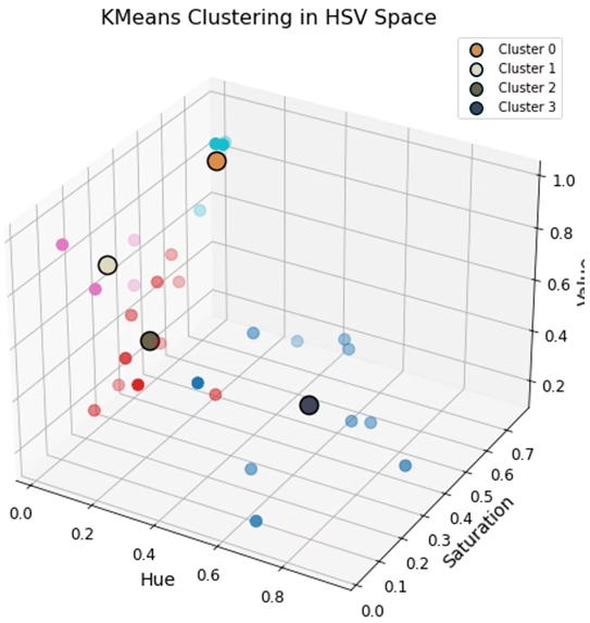
The histograms show that a majority of hues fall below 0.2, and that many paints are low in saturation or value. K-Means confirms this, but adds contextual structure: instead of simply knowing many paints are low in value, we now see that some form distinct clusters with low hue and low value (Cluster 2), or low hue and high value (Cluster 1). Furthermore, K-Means isolates a group of higher-hue paints (Cluster 3: greens, blues, violets), helping visually separate the small number of outliers that the histogram alone wouldn’t emphasize.
Conclusion
Through this analysis, I’ve gained a clearer understanding of my color palette and how my paints naturally group into four distinct clusters. While this structural insight is helpful, it also led me to rethink my assumptions.
Previously, I believed I had made a mistake by buying too many browns and other warm tones—colors that seemed to overcrowd the lower end of the hue spectrum. But this process reminded me of something important: I bought those colors because I needed them. They served a purpose in the models I painted, even if they didn’t balance perfectly in a color wheel or clustering plot.
So rather than rushing to “fill gaps” in the HSV space or buying new colors just to create a more even or aesthetically pleasing distribution, I now see more value in embracing the palette I already have. The goal shouldn’t be to force a sense of order, but to find it in what already works for me.
Looking ahead, I plan to build on this approach in a more practical way. In my next post, I’ll analyze the color compositions of paintings, miniatures, or real-world references that I find visually compelling. By extracting the color distributions from those images, I hope to identify which tones are actually beneficial additions to my palette.
If you read this far, and have questions on how I made these graphs, do contact me here.
Florius
Hi, welcome to my website. I am writing about my previous studies, work & research related topics and other interests. I hope you enjoy reading it and that you learned something new.
More Posts